Tracing Near Longest Paths with BPC Logic Filter

This article highlights the creation of a new targeted report from BPC Logic Filter to identify the “Near Longest Paths” of a project.

While BPC Logic Filter was originally developed as a pure logic tracer, I added a few targeted reports early on to reflect some specific needs, including the “Longest Path Filter” and the “Local Network Filter.”  This article highlights the creation of a new targeted report to identify the “Near Longest Paths” of a project.

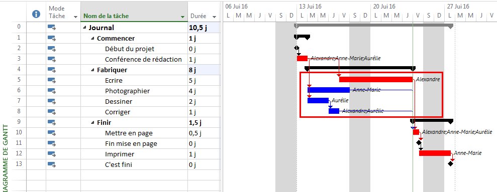
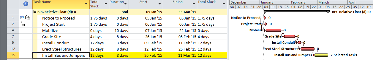
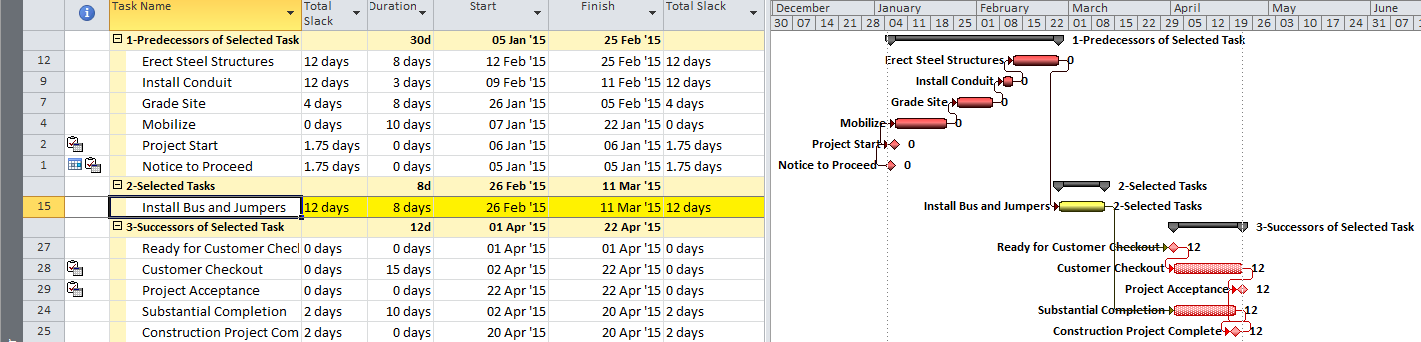
Often, when presented with a new project schedule in Microsoft Project, my first step (in concert with a logic health check) has been to run a Longest Path Filter analysis using BPC Logic Filter.  This report quickly and clearly identifies the driving path to project completion.  While the resulting filtered task list is useful for reporting, it rarely satisfies the needs of a serious analysis.  The second step, therefore, is to identify the associated near-longest-paths of the project by running a “Task Logic Tracer” predecessor analysis – with a positive relative float limit – for the project completion task.  The result is a clear description of the driving and near-driving paths to project completion.  The latest release of BPC Logic Filter adds a specific command to combine these two actions and generate a single “Near Longest Path Filter” for the project.

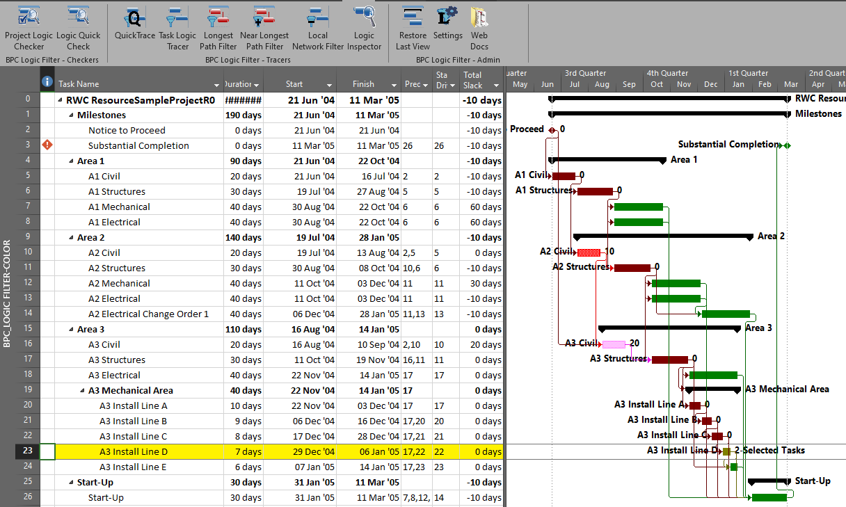
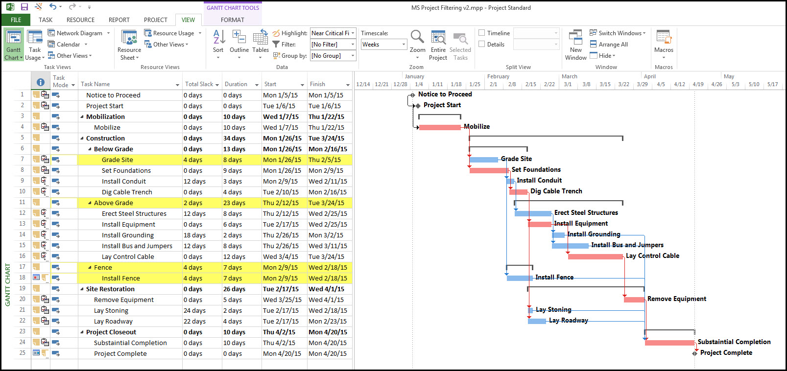
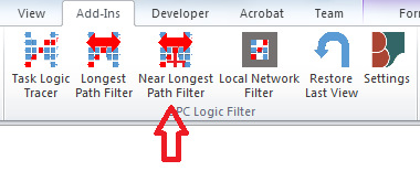
The mechanics are pretty simple.  As usual – with a Gantt view active in a project that contains logic – just open the Add-Ins ribbon [changed to the BPC ribbon in subsequent versions] and click on the button for “Near Longest Path Filter.”

bpclogicfilter-ribbongroup1611

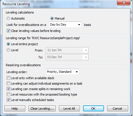
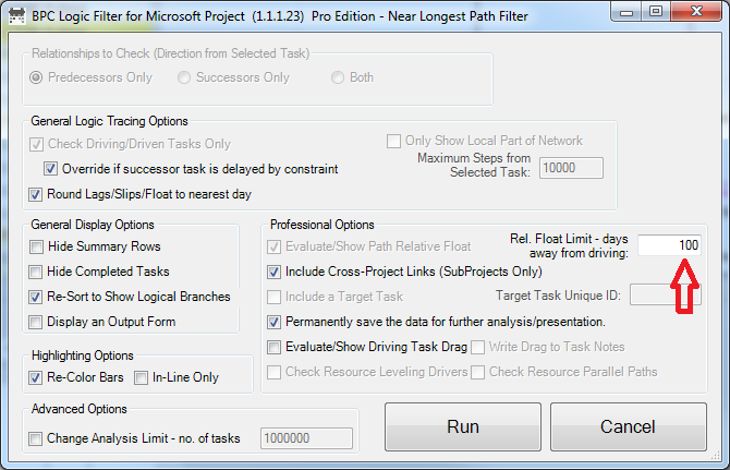
The add-in will initialize, and the user is given a choice of modifying the default analysis parameters.  Some of the parameters are pre-set and can’t be changed here.  The key parameter for a formal Near-Longest-Path analysis is the Relative Float Limit, highlighted below.  Any related task with a Path Relative Float that is less than the specified limit will be included in the filter; all others will be ignored and considered unrelated.  The default value is 100 days away from the driving/longest path (which can be changed in the Settings).

bpclogicfilter-near-longest-path-window

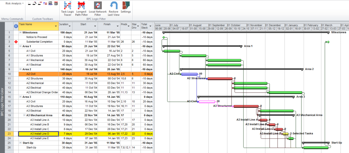
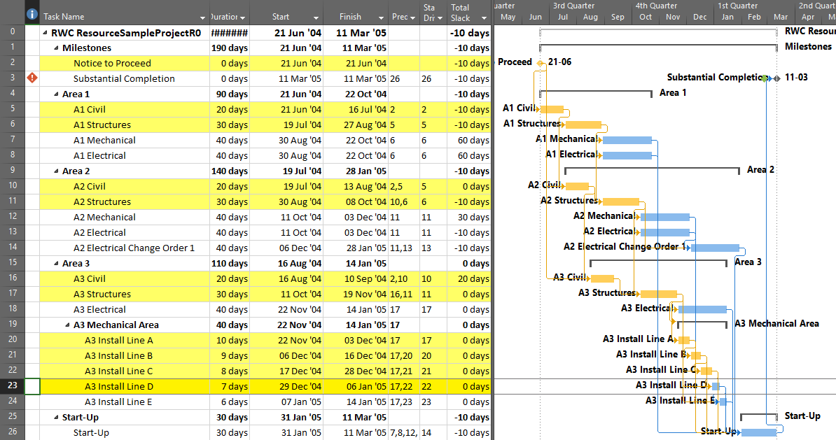
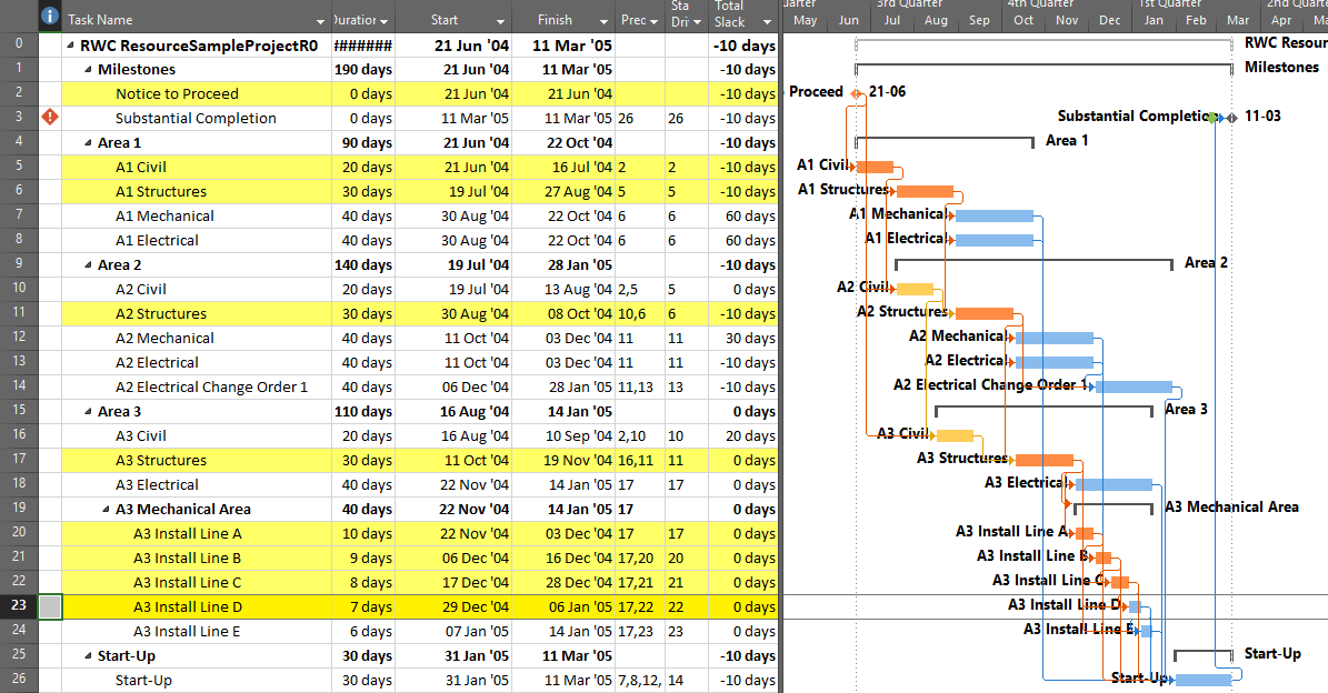
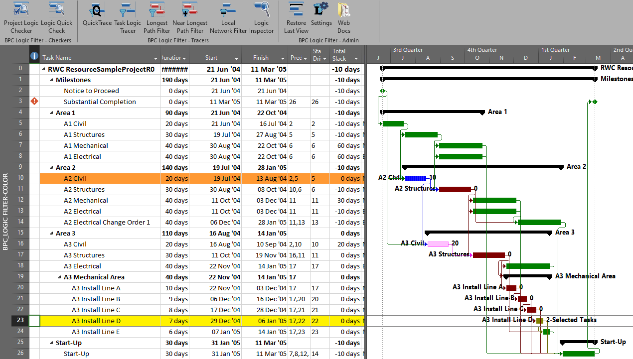
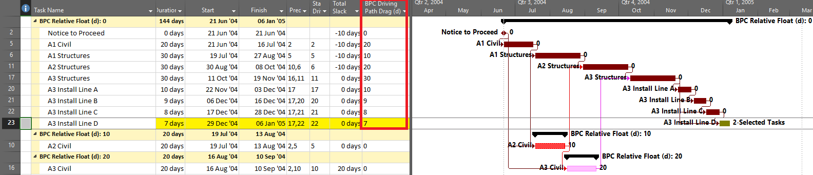
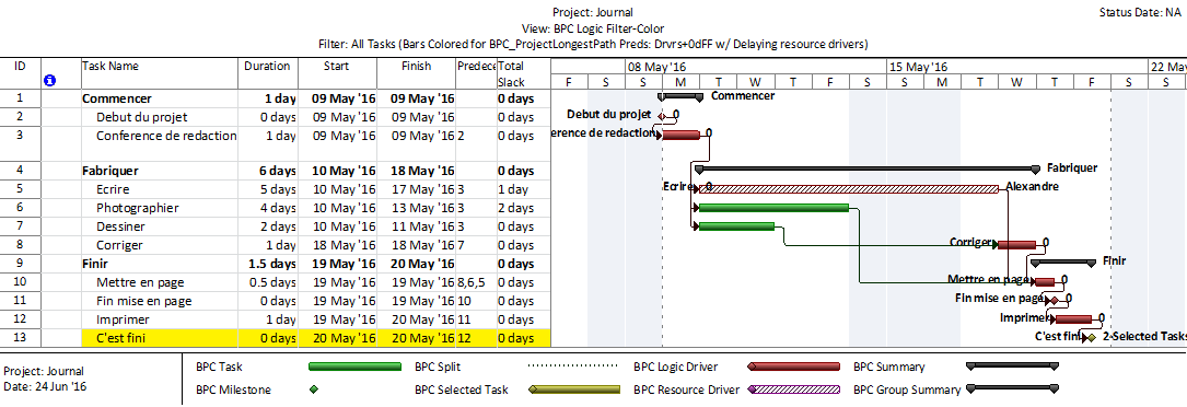
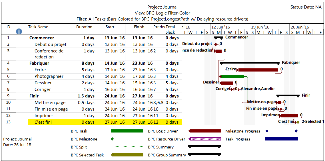
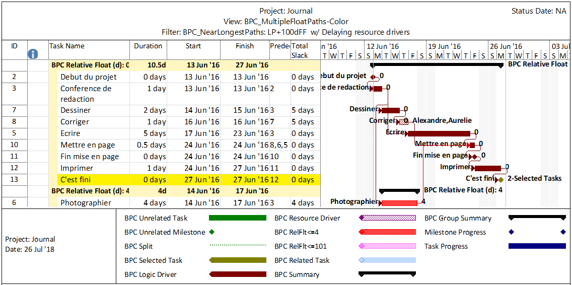
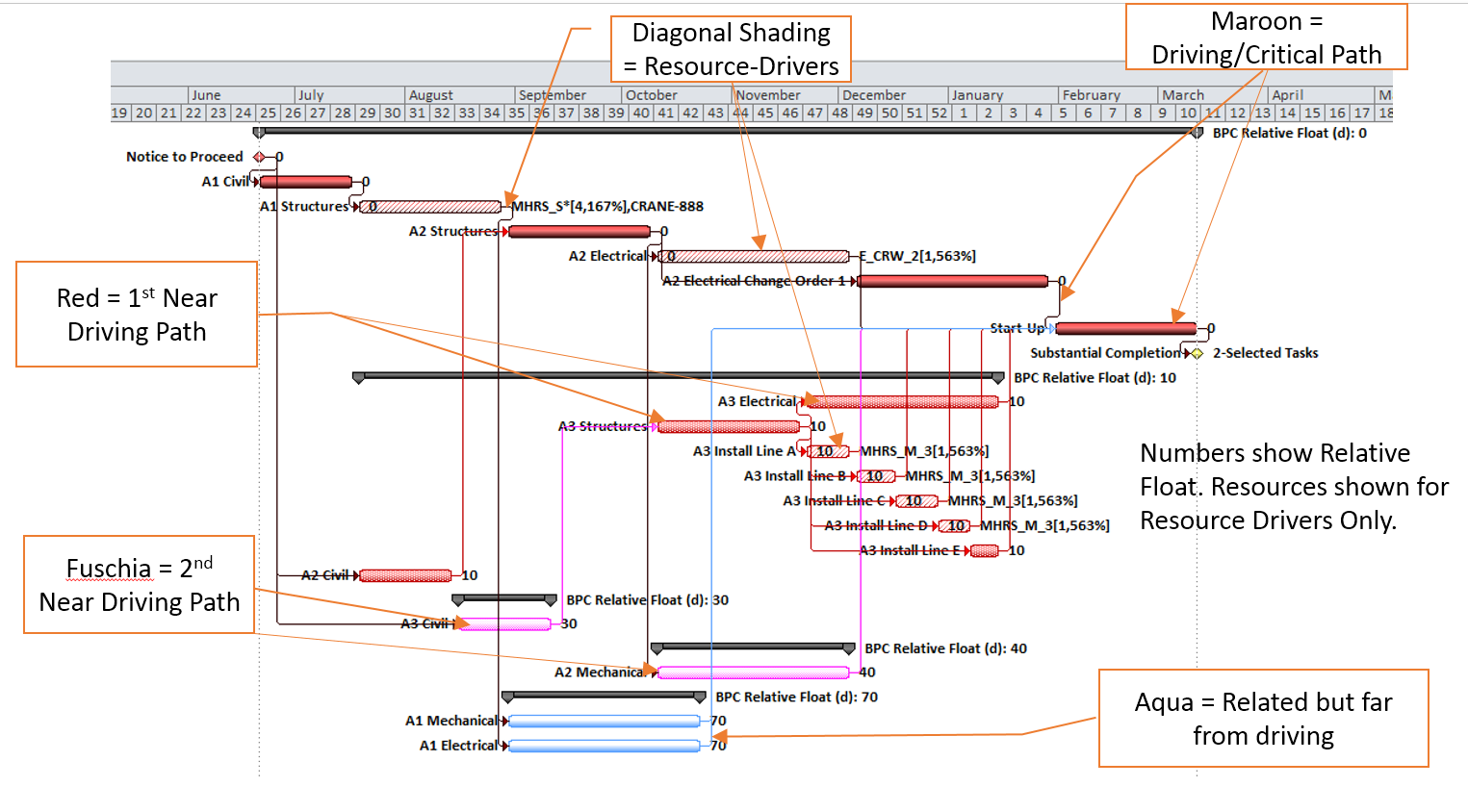
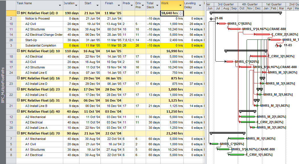
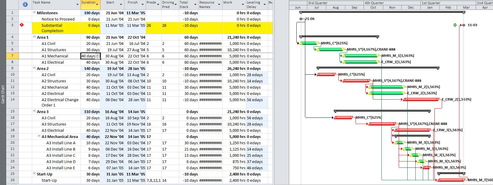
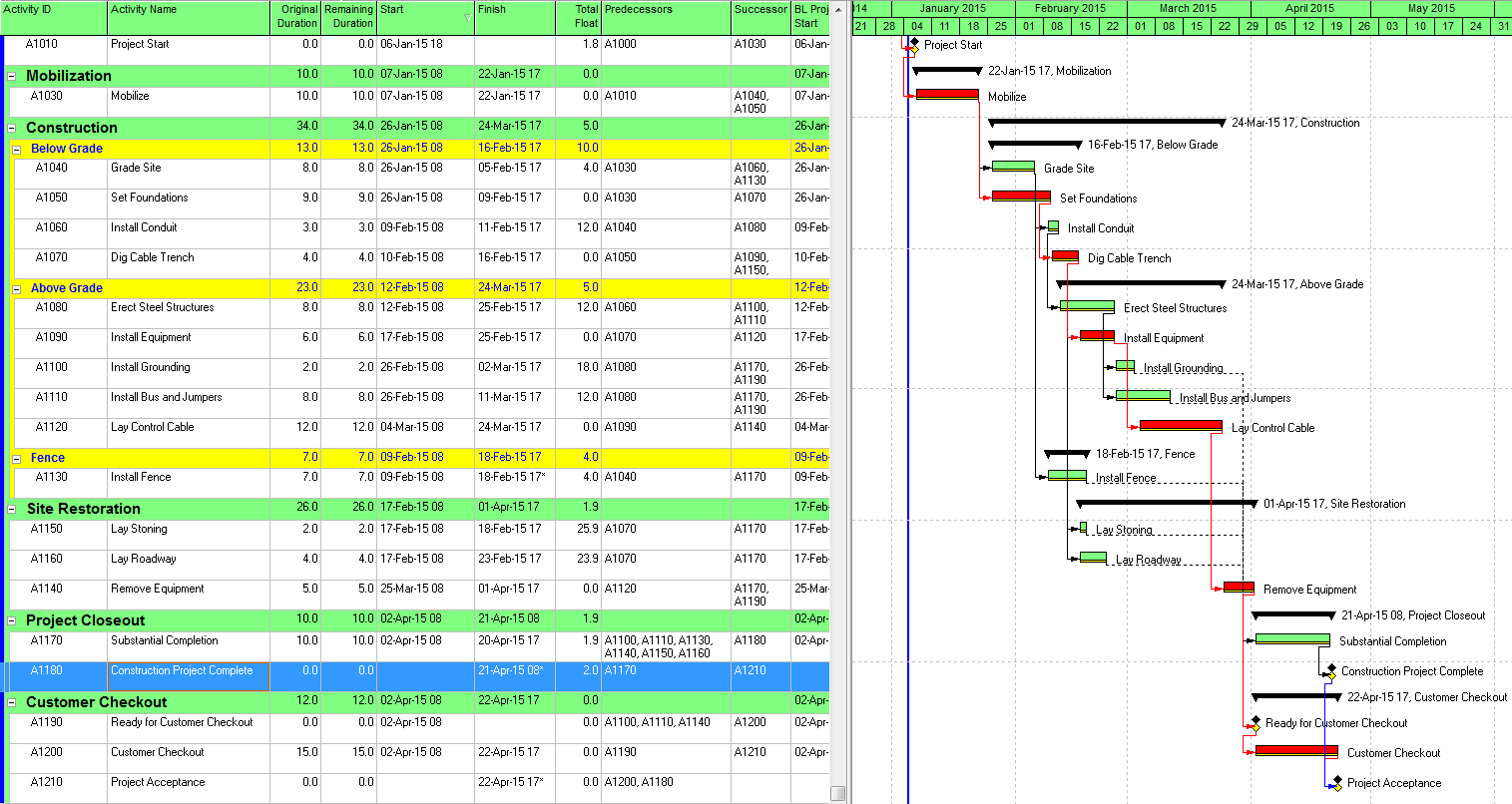
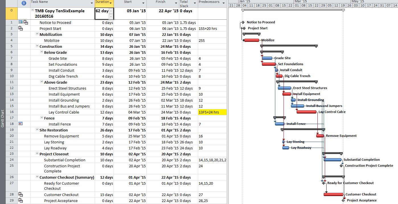
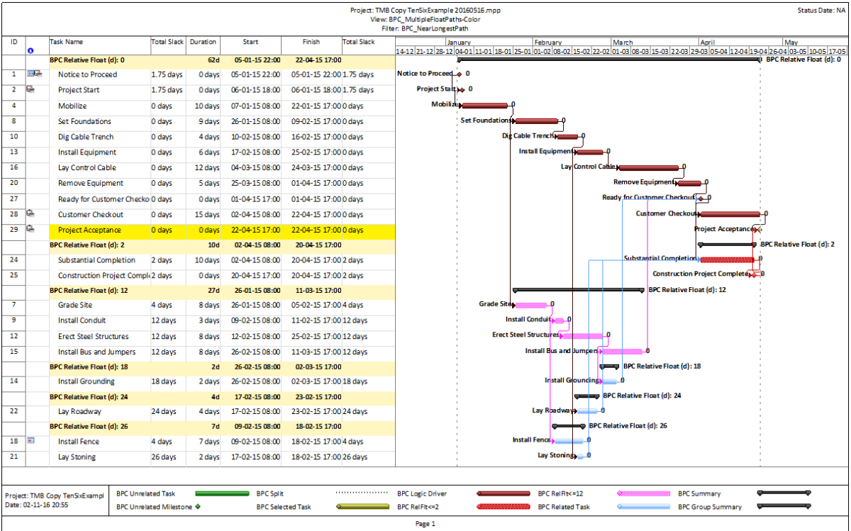
The standard output for a simple project (using the parameters selected above) is provided here.  Selecting “Re-Color Bars” instructs the add-in to generate the custom output shown, including the header, the legend, and five different bar colors depending on proximity to the Longest Path.  Thresholds for applying these bar colors can be manually adjusted in the program settings or, if desired, automatically adjusted by the add-in.  nlp_tensixexampleltr

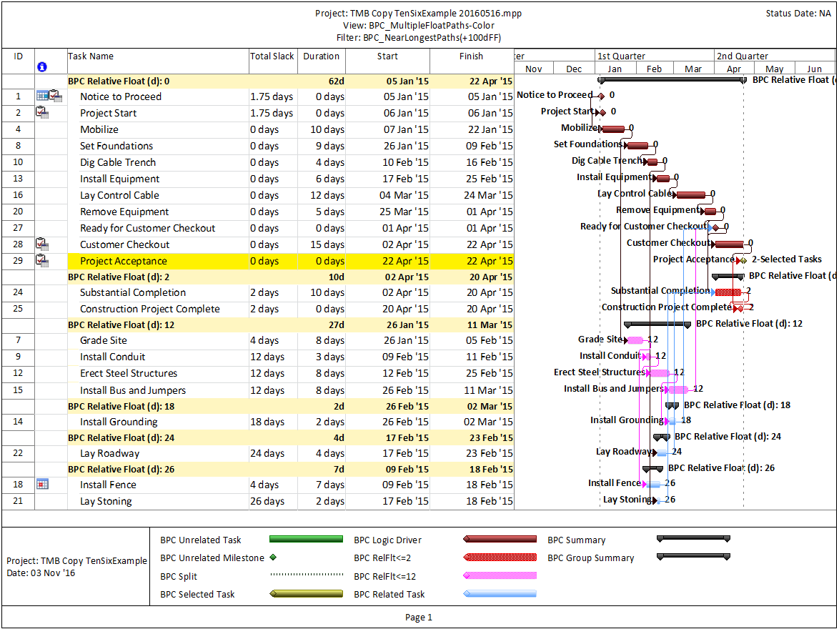
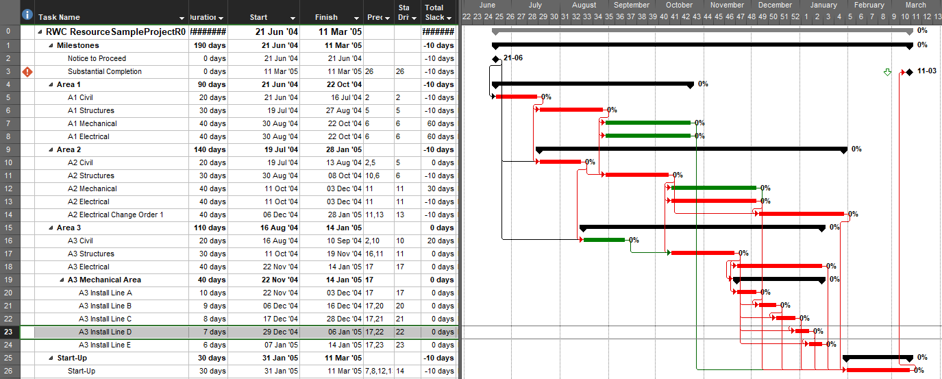
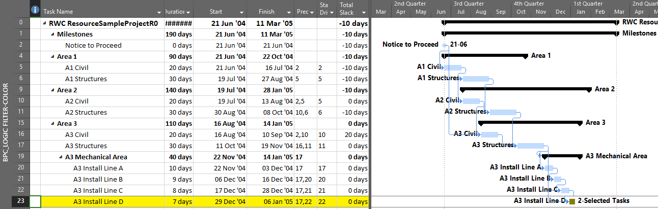
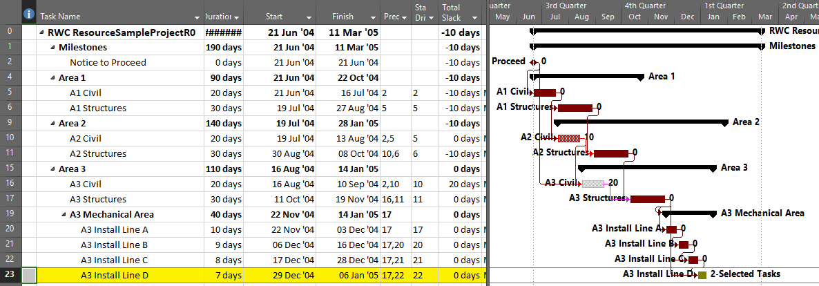
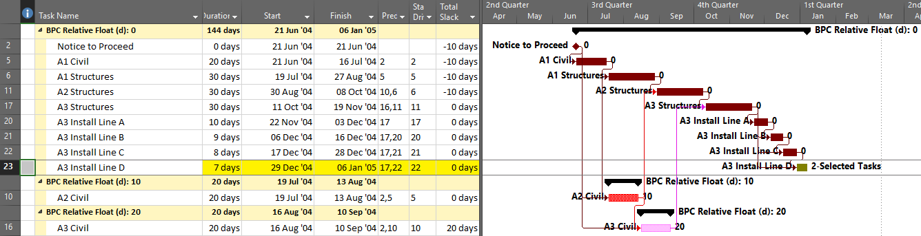
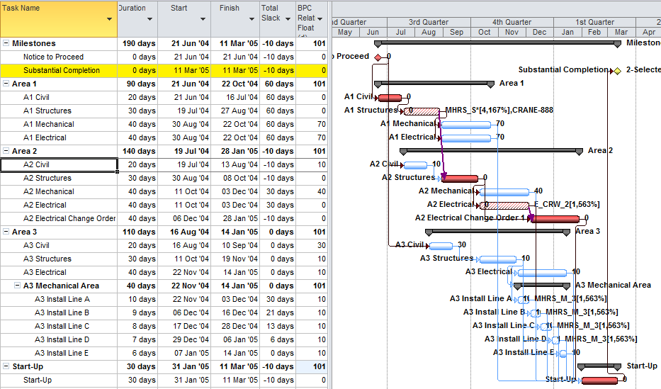
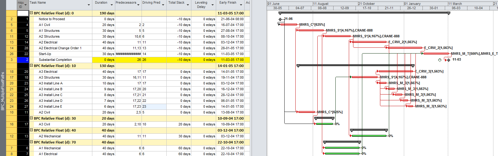
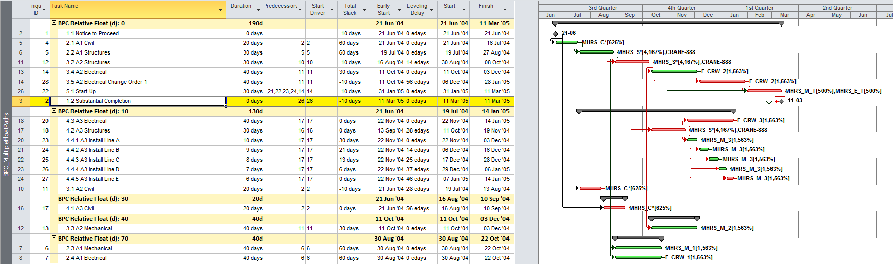
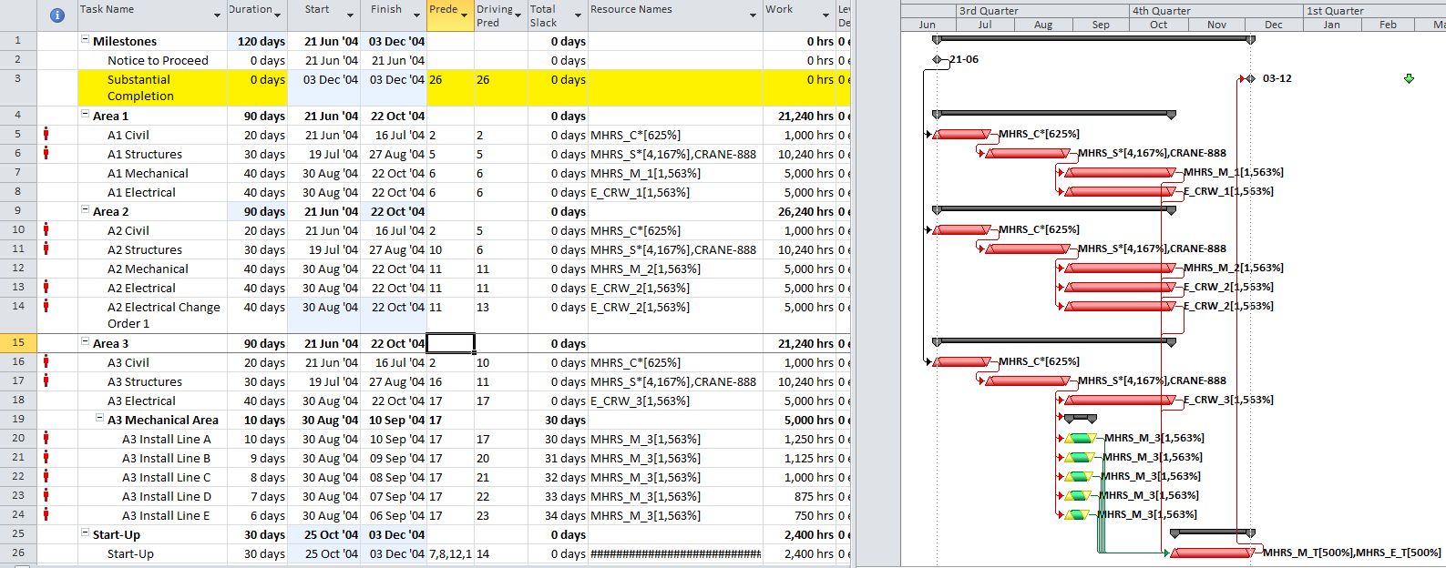
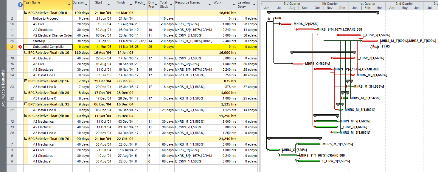
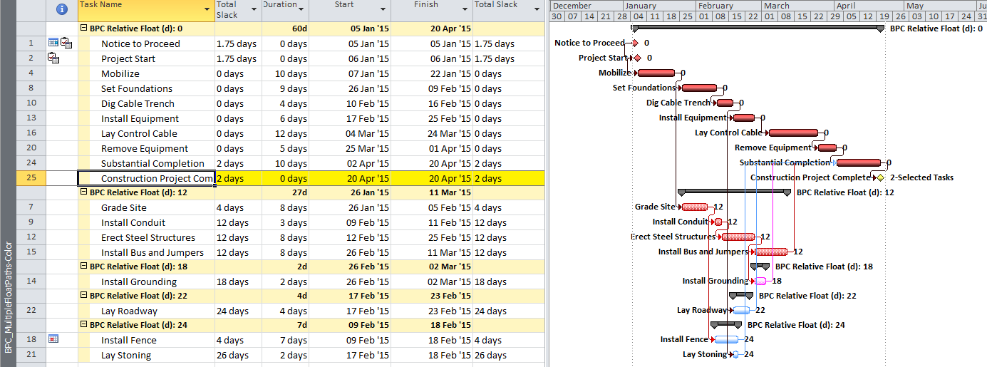
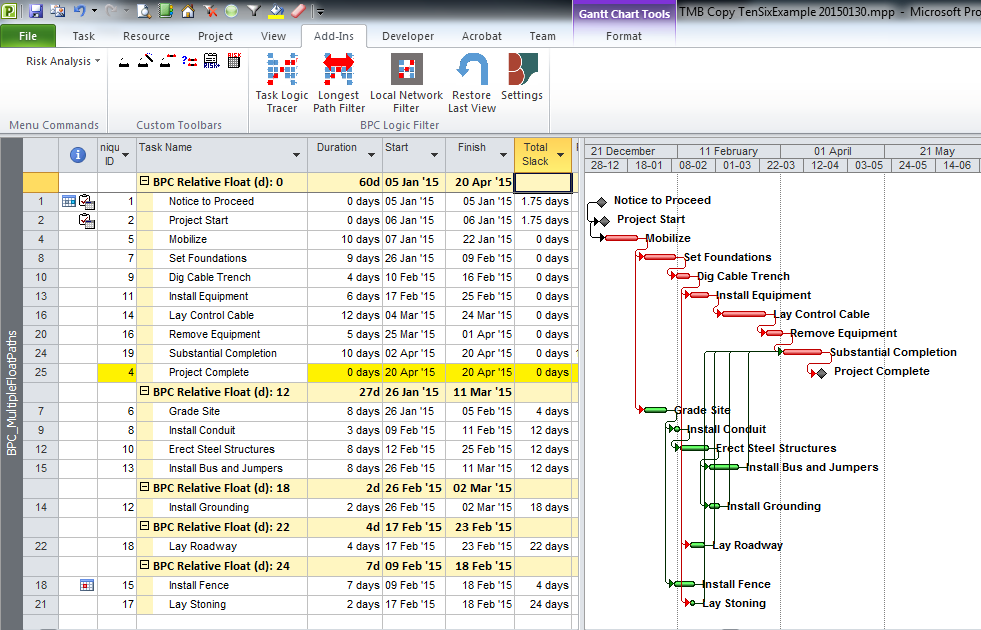
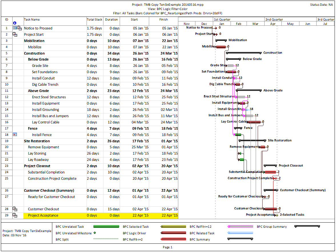
Here’s an alternate view showing the Near Longest Paths in-line in the context of an existing Outline/WBS organization.  In this analysis I reduced the Relative Float Limit from 100 to 20 days, and the three tasks at the bottom of the earlier figure were ignored.  Here they are given a green “BPC Unrelated Task” bar.

nlp_tensixexampleinlineltr

While I’ve always hated redundant work, this particular improvement to BPC Logic Filter was kick-started by my recent review of the draft of “Analyzing Near-Critical Paths,” a pending Recommended Practice from AACE International.  The new draft recommended practice is based largely on the previously-published (2010) Recommended Practice 49R-06 – Identifying the Critical Path.  According to both documents, Critical- and Near-Critical paths may be identified on the basis of total float/slack thresholds (in the absence of variable calendars, constraints, or other complicating factors) and – when total float/slack does not suffice – “closeness to the longest path.”  For the latter cases, 49R-06 suggests two methods of analysis:

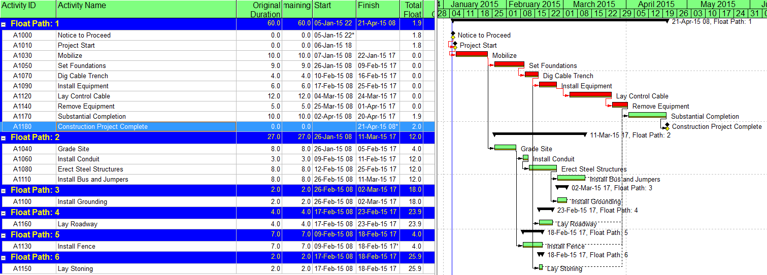
  • Longest Path Value – a metric that appears similar to Path Relative Float (in BPC Logic Filter) for the project completion task. This metric has been applied as an add-on to Oracle Primavera scheduling tools: See Ron Winter’s Schedule Analyzer.
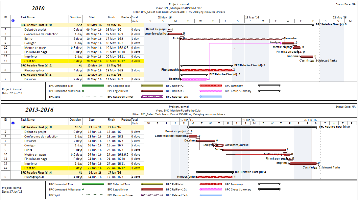
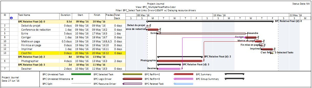
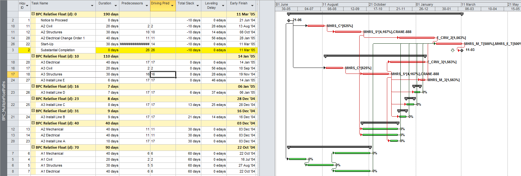
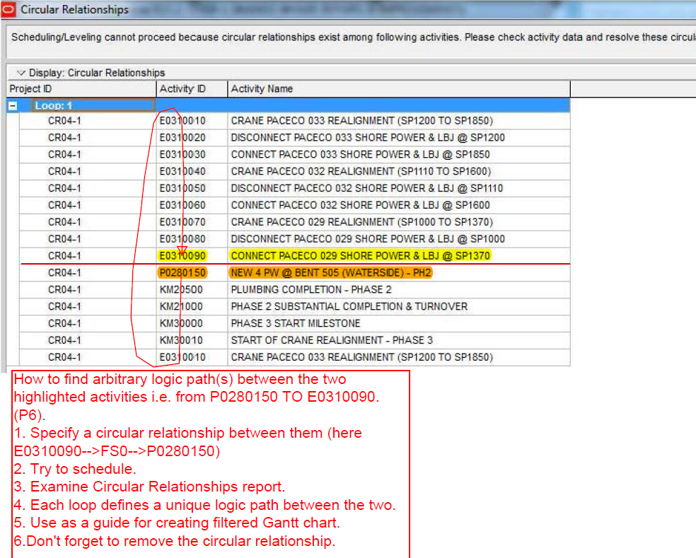
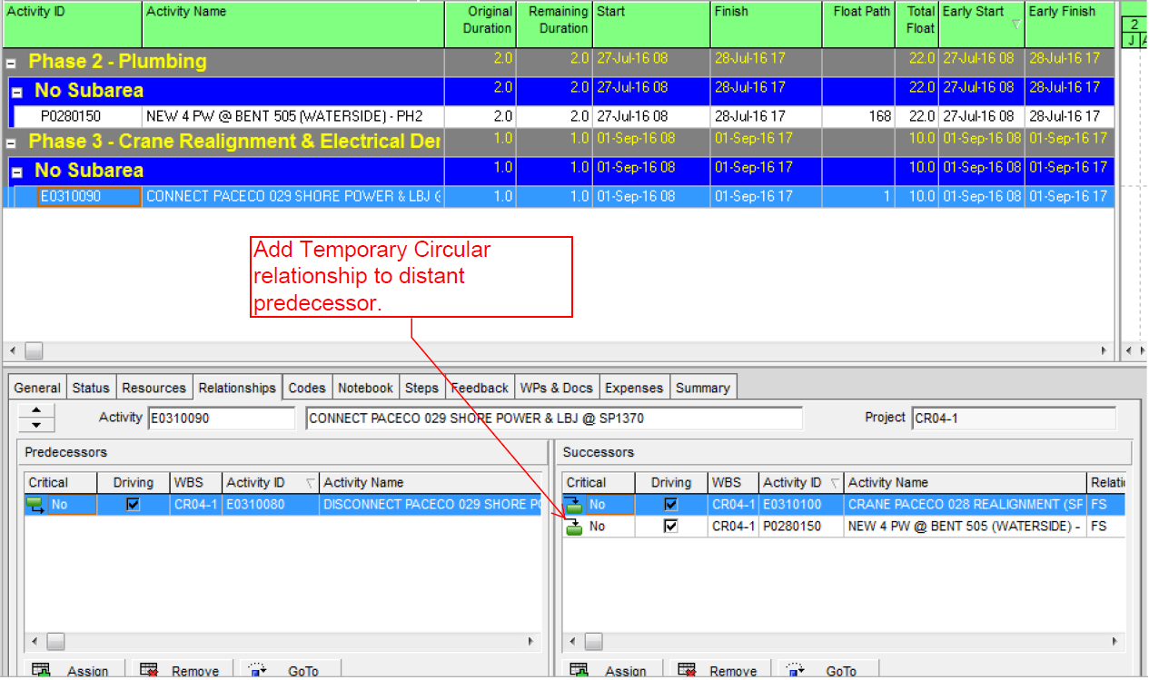
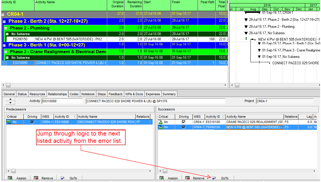
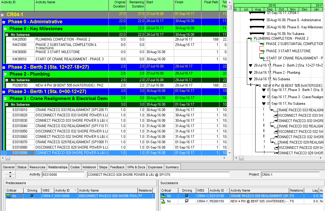
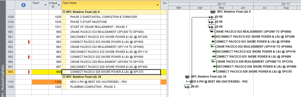
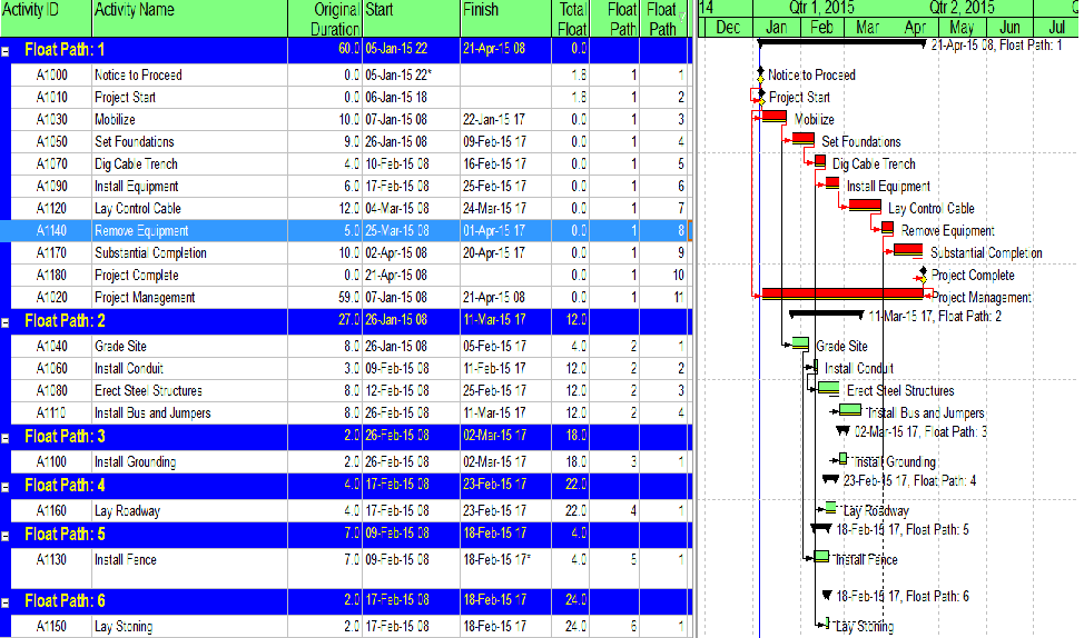
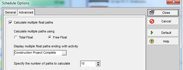
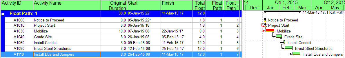
  • Multiple Float Path analysis. Like the Longest Path Value, Multiple Float Path analysis is primarily associated with Oracle’s Primavera scheduling tools – it is presented as an advanced scheduling option in P6.  As I’ve noted in Beyond the Critical Path – multiple float path analysis indicates closeness to the longest path without explicitly measuring and presenting it.  Detailed examination of the results, including relationship free floats, is necessary to determine the apparent relative float of each activity.

From its start, BPC Logic Filter has supported a similar analysis for Microsoft Project schedules through its Path Relative Float metric, Multiple-Float-Paths views, and other reporting.  The new “Near Longest Path Filter” offers a single-step approach to identifying and analyzing near-critical paths in the presence of variable calendars, constraints, and other complicating factors – when Total Slack becomes unreliable as an indicator of logical significance.

See also Video:

Video – Analyze the Near-Longest Paths in Microsoft Project using BPC Logic Filter


A Logic Tracing Example in Microsoft Project

This article uses BPC Logic Filter to present the progression of a single logic tracing example from a simple approach to a more focused analysis. [June 2020: revised for updated versions of MS Project and BPC Logic Filter.]

[If you came here looking for a simple logic tracing macro and are comfortable using Visual Basic for Applications (VBA), have a look at these two other entries: Macro for tracing filtering and sorting task paths in Microsoft Project and Simple Macro for Listing Driving Predecessor(s) in MS Project.  They may give you what you want as long as your project has simple logic.]

BPC Logic Filter is an excellent tool for defining and visualizing the Critical Path and Near-Critical Paths of a project when Total Slack proves inadequate – namely in the presence of constraints, variable calendars, and resource leveling.  As I’ve written elsewhere, however, the first version of BPC Logic Filter was prompted by a very different, though straightforward stakeholder request: “My people can’t see why they need to finish these tasks so soon. Isn’t there a report or something to show what other tasks (in other departments) are depending on them?”  In other words, couldn’t I group, filter, and sort tasks simply according to logical relationships – in addition to Work Breakdown Structure, responsible department, and other codes.  At its core, the resulting solution was a simple logic tracing routine for exploring, marking, and displaying logical relationships in an existing project schedule.

This article presents the progression of a single logic tracing example from a simple approach to a more focused analysis.

Consider the example of the small installation project presented below. There is a deadline on the “Substantial Completion” milestone, and the project is 10-days behind schedule. For unrelated reasons, the project manager has identified a need to examine the predecessor and successor logic paths around one task – “A3 Install Line D” – which is selected in the figure.


Task Inspector

We can first examine the task’s dependencies using MSP’s Task Detail Form and the Task Inspector pane.  The form shows that the task has two finish-to-start predecessors and two finish-to-start successors, but it provides no other schedule information for these dependencies.  Task Inspector identifies the second predecessor — ID 22 – A3 Install Line C — as the driving predecessor.  That is the predecessor whose logic is controlling the start date for our task.

This driving predecessor is hyperlinked, so clicking on it automatically selects the corresponding task in the task table and updates the details.  In addition, a new “Go back to” task link is added to the Inspector pane.  Starting from a specific ending task, the user can use these tools to “click-trace” backwards and forwards along the driving predecessor logic path to the selected task.

Click-tracing of driven successor paths is not possible using the Inspector pane, and predecessors that are hidden by filtering or outlining can’t be traced.  Moreover, neither external links nor resource-driving links can be traced.  Finally, the driving predecessors can be incorrect when relationships other than finish-to-start are used.

BPC Logic Filter – Task Logic Inspector

The Logic Inspector in BPC Logic Filter presents consolidated views of a task’s driving and non-driving predecessors and successors, including other relevant information like dates, resources, or user-selected fields.  Driving relationships are highlighted and listed at the top, while links to inactive predecessors are de-emphasized and listed at the bottom.  For logical significance, the ERF column indicates how far (in days) the predecessor is from controlling/driving the successor’s early dates, and the LRF column indicates how far the successor is from controlling/driving the predecessor’s late dates.  The latter is most useful when click-tracing to explore successor logic paths.  (The yellow-on-red color scheme in the figure highlights relationships that are driving in both directions.)

With the Jump buttons in the Logic Inspector windows, users can click-trace logic paths forward and backward through the project schedule.  Unlike the built-in tools, the Logic Inspector windows allow inspection and click-tracing of both driving and non-driving logic along successor paths, external (i.e. master/sub-project) paths, resource-constrained logic paths, and hierarchical logic paths.

Task Paths and Task Path Filters

Recent versions of MS Project (2013+) include Task Path bar styles for graphically highlighting predecessor and successor paths on the Gantt chart.  In addition, it is possible to use a simple “QuickTrace” macro (like the one linked above or one of the freeware settings in BPC Logic Filter), to identify the same set of related tasks.  In the next figure, the Path Predecessors bar style has been applied to color the bars of all tasks that are path predecessors of the selected one.  The QuickTrace macro (included in BPC Logic Filter) has also been used to highlight the same related tasks.

Alternately, QuickTrace can display the related tasks using a filter rather than a highlighter, as shown below.  In either case, the actual driving logic for the selected task is not apparent.  (And no, Total Slack does not define driving logic for this task.)

The next figure displays both the Path Predecessors (orange) and the Path Driving Predecessors (red-orange) bar styles for the selected task, and QuickTrace has been used to highlight the driving predecessors in the table.  A corresponding filter could also be applied.

Although generally less useful for analysis, corresponding bar styles and filters can be applied for the path successors and path driven successors of the selected task.

BPC Logic Filter – Advanced Tracing

With advanced logic analysis features, the relative float of all the predecessor task paths can be defined and displayed.  The following chart shows the entire project, with the predecessor paths of the selected task highlighted according to their path relative float in days.  (Path relative float indicates how much a particular task or path may be delayed before affecting the selected task; i.e. “days away from driving”.)  Path relative float is indicated numerically at the right side of each related bar.  Unrelated bars are de-emphasized and colored green.  The bar chart shown is similar to that obtained using the Task Path bar styles, with the key exception that non-driving predecessor paths can be ranked.

BPC Logic Filter allows one variation – bounded network analysis – to only show connections to a particular target task.  The figure below highlights the connections between the selected task, A3 Install Line D, and the target task, A2 Civil.

The previous two figures displayed the related task paths in-line and within the context of the overall project view.  A more focused view of the driving and near-driving paths is provided by applying a filter to hide all unrelated tasks, as shown here.

It is often useful to group and sort tasks to clearly display the chain of driving logic and associated near-driving paths.  The first group in the figure below – “BPC Relative Float (d): 0” – indicates the driving logical path for the selected activity.  The next two groups depict branching logical paths (one task each) that are 10- and 20-days away from driving the selected task.

Finally, when attempting to accelerate a task by shortening its driving logical path, Drag quantifies the maximum acceleration that may be gained by shortening a particular task along that path.  Drag is limited by the existence of parallel paths, as clearly evidenced by Tasks 6 and 11 in the figure below.  For focused acceleration of complex projects, the Drag metric can assist in prioritizing actions.

The examples shown here represent successively more powerful analyses of driving logic for an arbitrary task in a project schedule.  If that task were the final task or a key completion milestone for the project, then the resulting special case of the driving path would be the “Critical Path” for the project.

See a related video entry:

Video – Logic Tracing Example in Microsoft Project


Musings on Critical Path Drag and Calendars in CPM Schedules

As is the case for Total Float/Slack, introducing variable task calendars can significantly confuse the understanding of Critical Path Drag in Project Schedules.  

[See also Simple Macro for Computing (Duration) Drag in MS Project and

Video – Compute Critical Path Drag in Microsoft Project]

Critical Path Drag is a useful metric in CPM scheduling that Stephen Devaux introduced in his book Total Project Control, but it is not widely computed or used.  Drag represents the individual contribution of any single schedule element (e.g. a task) to the overall duration of a project.  By definition, only “Critical Path” tasks have it, and a task’s Drag indicates the total theoretical project acceleration that could be gained if the task’s remaining duration were reduced to zero.  Viewed simplistically another way: if Total Float/Slack represents how much a non-critical task may slip before becoming Critical; Critical Path Drag represents how much a Critical task may be compressed* before becoming non-Critical.  This can be very useful in focusing a project acceleration (e.g. Crashing) exercise.

It’s clear that theoretically many components in a CPM schedule can possess Drag: activity durations, early constraints, and predecessor lags to start with. Activity calendars can also possess Drag.  I originally incorporated Drag analysis into BPC Logic Filter with the aim of correctly analyzing the Drag possessed by each component, but I recently decided to at least temporarily set aside that idea for the following reasons:

  • Drag seems so rarely used in practice that using even a single number for each activity is a stretch for the typical user; parsing it out to its many components seems unhelpful to most.
  • Allocating Drag purely by passive network analysis is hard.
  • Most importantly, other Drag-computing software (namely Spider and Asta) seem to compute only a single figure for each activity.  Allocating Drag to different components could conflict with these single-value metrics under some circumstances, leading to confusion and possible loss of confidence in the tool.

Now BPC Logic Filter provides an option to compute a single driving path Drag number for each task included in a logical analysis – using a brute-force, remove-and-recalculate approach.  This Drag reflects the maximum acceleration of the project’s completion milestone (or any other selected milestone or task in the project) to be gained by modifying the task’s duration alone.  A negative value indicates that the project is shortened by lengthening a particular task – this is reverse logic flow.

As is the case for Float/Slack, introducing variable task calendars can significantly confuse the understanding of Drag.  Consider a simple project comprising three 1-day tasks in sequence, beginning on a Friday and with the first two tasks assigned the “Standard” calendar, i.e. 5dx8h. The concluding task “Activity 3” (perhaps a management task) is on a “Monday-Only” calendar.**  As shown in the figure below, Activity 3 is scheduled to complete on the second Monday.***   Clearly, removing the duration of Activity 1 (or 2) will accelerate the Completion Task – Activity 3 – by seven calendar days, from the second Monday to the first Monday.

spiderdragex

So what is the Drag of Activity 1?  As shown by the combined figures below, the answer depends on the calendar used to quantify the acceleration.  Measured according to Activity 1’s own calendar, a Monday-to-Monday acceleration is 5 days – indicating 5 days of Drag.  That same Monday-to-Monday acceleration is only 1 working day according to the calendar of the Completion Task – resulting in 1 day of Drag.  Using the Project’s overall calendar could provide different results altogether.  For Activity 3 of this example, the Project Calendar is neither the Local Task Calendar nor the calendar of the Completion Task (also Activity 3); then it becomes like the first two tasks with a Drag of 5 days.

dragcal

Which is the correct calendar to use?  My own preference is to use the calendar of the Completion Task to quantify potential acceleration of the Completion Task (i.e. the middle option above), and this is the default selection in BPC Logic Filter. A detailed logical analysis would assign 1 day of Duration Drag to each of the tasks in the example and a further 4 days of Calendar Drag to Activity 3.  There is no logical basis for adding these 4 days of Calendar Drag to any other task, but using a mismatched calendar in a brute-force Drag analysis does exactly that, as shown in the top and bottom options above.  Those options remain in BPC Logic Filter to allow consistent comparisons with Drag calculations from other tools.

*In the absence of constraints, variable calendars, and certain relationship lags; the compression of a particular Critical Path task can lead directly to compression of the project.  Then the idea that Drag represents the potential productive compression of the task itself (i.e. the mirror image of Total Float/Slack) can appear true.  Such a simplified view should not be generalized for complex projects, however.  

**Credit and thanks for this example go to Vladimir Liberzon of Spider Project.  Spider is one of the few scheduling tools to compute Drag.

***Project correctly computes Total Slack of 4 days for the first two tasks, meaning they could each slip 4 days – according to their own calendars – without delaying the project.  MSP marks them non-Critical.  They are nonetheless on the driving path to project completion, as shown by BPC Logic Filter, and they possess Drag.


Leveling Changes from MSP 2010 to MSP 2013

[I’ve slightly edited this old article – mostly figures.  After “upgrading” to Microsoft Project 2016, I can confirm that MSP 2016’s resource leveler appears similar to MSP 2013’s leveler in the simple case examined; both are substantially different from MSP 2010’s.]

Over the last few years, some tests of resource leveling algorithms in various software packages have been reported informally over at Planning Planet.

When using “default” conditions (i.e. without implementing any user-defined priority schemes), the general picture was that leveled schedules from MSP 2010 were significantly longer than those from MSP 2007.  There have also been reports that MSP 2013 (and MSP 2016, which seems to use the same leveling rules) produces even longer leveled schedules than MSP 2010.  Other software (Spider Project in particular) tend to produce shorter schedules under resource constraints.  I haven’t paid too much attention to these reports because a) I don’t use resource leveling often, and b) when I do use leveling, I always define some specific leveling priorities, so the “default” results are not so relevant.

Last week, a French planner (“Alexandre”) on PP noted some significant changes in default leveling results when migrating a simple schedule from MSP 2010 to MSP 2013, wondering what might be the reason for the changes.  I’m still on 2010, so I haven’t noticed the change in 2013.  While it’s clear that Microsoft has modified the leveling rules from version to version, they don’t publish the details, so addressing the “reason for the change” is just speculation.  My own speculation is that minor changes to the leveling algorithm were made to limit apparent changes to the pre-leveling “Critical Path,” even at the expense of extending the schedule.  For Alexandre’s specific example:

  • The project has a total duration of 7.5 days, and the pre-leveling (i.e. CPM) critical path runs through task 5.  Task 5 has 0 days of total slack, while task 8 has 2 days of slack.
Leveling Fig0
Figure 0. Pre-Leveling (CPM) Schedule – 2010
  • In resolving the resource conflict between task 5 and task 8, MSP 2010’s default rule gives greater scheduling priority to task 5 because:
    • The CPM schedule has it starting earlier;
    • It has lower total slack in the CPM schedule;
    • It has a longer duration;
    • It comes first on the task list;
    • It is marked as “Critical” (?);
    • Some other factors…(?).

(I have no idea what the relative contributions of these factors are in the scoring.  Some might be zero.)

    • As a consequence of leveling, task 5 (the “critical” one) is scheduled first, while task 8 is delayed, and the project is extended 1 day for a total duration of 8.5 days. Total slack is re-computed after incorporating the leveling delays, and a new “Critical Path” is displayed.
      • Perversely, Task 5 – which was clearly “critical” before leveling and is also clearly a resource driver for the project completion – now has 1 day of Total Slack.

        Leveling Fig1
        Figure 1. Leveled Schedule – 2010
      • Task 7 is now shown as “Critical,” even though there is neither a logical nor a resource-driving reason justifying it.
      • So in short, the MSP 2010 leveling algorithm can substantially change the “Critical Path,” and the resulting slack values can be completely misleading. (I wrote about this here: Logic Analysis of Resource-Leveled Schedules (MS Project).)
      • The next figures (from BPC Logic Filter) illustrate the actual resource-constrained Longest Path (Fig. 2) and Multiple Float Paths (2a) through the 2010 schedule.
Leveling Fig2
Figure 2. Resource-Constrained Longest Path of Leveled Schedule – 2010
Resource-Constrained Multiple-Float Paths of Leveled Schedule - 2010
Figure 2a. Resource-Constrained Multiple-Float Paths of Leveled Schedule – 2010
  • In contrast, MSP 2013 task gives greater scheduling priority to task 8, delaying task 5. I suspect this is driven by some complex tuning of the leveling rules around Total Slack.
    • Alexandre provided the MSP 2013 leveled schedule here (which also includes a minor date shift).

      Leveled Schedule - 2013
      Figure 3. Leveled Schedule – 2013
    • I’ve repeated it below in my [MSP 2016 model using Standard leveling order.]  The resulting “Critical Path” appears essentially the same as the pre-leveling version, but with an added 3-day leveling delay before task 5. This may give project managers confidence that the leveling exercise has not “screwed up” their critical path.
      Figure 4. Leveled Schedule – 2016

      Unfortunately, the project finish has been extended by an additional 2 days compared to the MSP 2010 leveler.  It is now 10.5 days.

    • The project manager’s confidence in the critical path is still misplaced. Task 7 and task 8 are now shown as far from critical, with 5 days of total slack.  As shown in the next two figures from BPC Logic Filter, however, they are obviously on the resource-constrained longest path through the schedule.
Figure 5. Resource-Constrained Longest Path of Leveled Schedule – 2016
Figure 5a. Resource-Constrained Multiple-Float Paths of Leveled Schedule – 2016

Comparing the 0-Float Paths of the two schedules (Figures 2a and 5a), we see that unlike MSP 2010, MSP 2013 and MSP 2016’s leveling engine has preserved the logic drivers from the pre-leveling CPM schedule while implicitly inserting task 7 and task 8 into the driving path to project completion.   Although the project is extended as a result, the appearance of a stable critical path is preserved.  Fortunately, BPC Logic Filter depicts the resulting resource-constrained critical path clearly in both cases.

My speculation on the reason for the changed algorithm is based on the Project development team’s demonstrated preference for the appearance of stability (for mid-level users) over behavior that might be more technically correct from an advanced user’s point of view.  (See the handling of inactive tasks in MSP 2013 for another example.)

For an update on this topic, see Resource Leveling Changes from MSP 2010 to MSP 2016 – Revisited


Eddies and Checkdams: Odd Structures in CPM Logic Flow

In logic-driven project schedules, the scheduled start and finish of each activity is determined by a “driving path” of predecessor activities and relationships.  Driving logic is said to “flow” along this path from the earliest predecessor to the activity’s completion.  In simply-modeled projects, this driving logic flow is one-directional and continuous, such that any delay (or acceleration) of a predecessor task is directly translated to a corresponding delay (or acceleration) of its ultimately driven successors.  Thus, delaying a task on the “Critical Path” (the driving path to project completion) ultimately delays the project.  More complex schedule models – i.e. those using other than finish-to-start relationship links – allow the driving logic flow to be checked or even reversed, so delay or acceleration of a given task may not have the anticipated result on other tasks or on the project as a whole.  Such effects can be transient, appearing and disappearing in the course of a single progress update.

Some Cases

Last year I read a series of articles by Miklos Hajdu (Research Fellow at Budapest University of Technology and Economics) on the sometimes-unexpected consequences of certain relationships in logic-driven project schedules.  I encountered them again a few months ago during an extended Linked-In discussion that Hajdu started relating to Drag calculation.  (BPC Logic Filter is one of the few scheduling tools that actually sets out to compute drag, and we identified some areas needing standardization of definitions.)

Hajdu’s Articles laid out five basic cases where incrementally delaying or accelerating a particular Critical Path activity might not lead to the expected delay or acceleration of the overall project:

  • Normal Critical Activities (Expected Behavior – i.e. Lengthening task extends project; Shortening task shortens project.)
  • Neutral Critical Activities (Neither lengthening nor shortening the task has any impact on project completion.)
  • Bi-Critical Activities (Either lengthening or shortening the task always extends the project.)
  • Reverse Critical Activities (Lengthening the task shortens the project; Shortening the task extends the project.)
  • Increasing Neutral Decreasing Reverse Critical Activities (Lengthening the task has no impact on project completion; Shortening the task extends the project.)
  • Increasing Normal Decreasing Neutral Critical Activities ( Lengthening the task extends the project; Shortening the task has no impact.)

A more recent blog by consultant Pat Weaver, Critical confusion – when activities on the critical path don’t compute…… reviewed these cases and illustrated the consequences using time-scaled-logic diagrams rather than the simple fragnet blocks first used by Hajdu.  With graphical images especially, Weaver has done a great job of clarifying the underlying logic flow and emphasizing the consequences of careless planning.  His article is a good read. Unfortunately, his suggestion that competent planners should avoid creating any such constructs in their project schedules seems impractical for planners using P6 or Microsoft Project to schedule complex projects.

I had encountered all of these issues previously in various project schedules and and had focused on them quite a bit while developing the drag-associated parts of BPC Logic Filter – that’s where the “Negative, Positive, and Absolute” terminology below came from.

Driving Logic Flow of the Cases

At the start of a project (i.e. ignoring progress updates and Data Date), every activity is scheduled to be completed according to a path of driving logic (comprising predecessor activities AND relationships) extending from the project start milestone or some valid external constraint forward to the activity’s Finish. (For the particular case of the Project Completion activity, its driving path is synonymous with the “Critical Path” of the project.)

  • Identifying the “Driving Logic Flow” through any arbitrary activity along that path starts with the Relationship Free Float values of its predecessor and successor links.  A Relationship Free Float value of 0 indicates a driving relationship, while a value greater than zero indicates a non-driving relationship.
  • The activity’s duration “participates” in the driving logic flow if (and only if) there are “Driven” and “Driving” relationships at opposite ends of the activity. Various combinations of relationship float have the implications in the table below.
Relationship Float and Driving Logic Flow

Keeping in mind that any changes to activity duration can immediately change the driving logic flow through the schedule and the associated relationship floats – such that an activity described by the first line of the table above may jump to the third line simply by adding a day to its duration – we can interpret the table as follows:

  • An activity with a Driven Start and a Driving Finish has a Positive duration participation, as the logic flows forward through the duration from Start to Finish.  This is “Normal” in Hajdu’s articles; lengthening the task extends the project, while shortening the task shortens the project.  This case seems to represent the vast majority of activities in typical schedules.  BPC Logic Filter computes a drag value corresponding to the activity duration, any applicable constraints, and parallel (i.e. near-critical) paths.

    Duration and Logic Flow1
    Positive Duration Participation in Logic Flow (“Normal Critical”)
  • An activity with a Driven Finish and a Driving Start, on the other hand, has a Negative duration participation, as the logic flows backward through the duration from Finish to Start.  This corresponds to Hajdu’s  “Reverse-Critical” case; lengthening the task and thereby allowing it to start sooner ends up shortening the project, while shortening the task and thereby forcing it to start later ends up extending the project.  BPC Logic Filter computes a negative drag value for these cases, partly to indicate the apparently perverse logic at work. While such tasks seem to be rare in baseline schedules, I have seen them arise during updating on fairly high-level integrated masters (i.e. not in construction).

    Duration and Logic Flow2
    Negative/Backward Driving Logic Flow through Duration – Starting Early and working slower Helps; Starting Later and working fast hurts.
  • For an activity with only a Driven Finish and Driving Finish (or Driven Start and Driving Start), then the duration is bypassed and has no participation in the driving logic flow.  This corresponds to Hajdu’s “Neutral Critical” case; neither lengthening nor shortening the task has any impact on project completion, and BPC Logic Filter computes a duration drag of zero for task B.  It should be noted that although “dangling starts” and “dangling finishes” are evident in the examples depicted below, they are unrelated to the zero-participation observed.  Adding non-driving start predecessors and/or finish successors to Activity B would not change the conclusions.
    Logic Flow Duration Bypass - Through Finish
    Logic Flow Duration Bypass – Through Finish

    Duration and Logic Flow3
    Logic Flow Duration Bypass – Through Start
  • An activity with both driving and driven relationships at both ends (i.e. minimum Relationship Float = 0 in all four columns of the table) represents four parallel driving logic paths:  1) through the Start only; 2) through the Finish only; 3) forward through the Start, the Duration, and the Finish; and 4) backward through the Finish, the Duration, and the Start.  In this case, the Duration Participation is “Absolute,” since any change to the activity duration (either positive or negative) results in positive (lengthening) of the overall path.  There is no chance to accelerate the project here, so BPC Logic Filter computes a duration drag of 0.  This case corresponds to Hajdu’s “Bi-Critical” case.  I’ve added an additional predecessor and successor to the illustration fragnets below – mainly to indicate that its occurrence is not limited to ladder-logic structures.  The combined “Positive” and “Negative” behaviors are obvious.

    Duration and Logic Flow5
    Absolute Participation = Positive/Normal on Lengthening, Negative/Reverse on Shortening
  • Finally, the four variations of “Limited” Duration Participation arise from the cases where three of the four “Relationship Float” columns are zero.  They essentially represent various combinations of “Positive,” “Negative,” and “None” cases above, and they correspond to Hajdu’s “Increasing Normal Decreasing Neutral” and “Increasing Neutral Decreasing Reverse” cases.   With any of these cases, it is only possible to Lengthen, never to Shorten, the overall length of the project by modifying the duration of Task B, so BPC Logic Filter computes a drag of zero.
    Duration and Logic Flow6
    Positive Limited Low Participation – Acceleration won’t help, but slippage will hurt.
    Duration and Logic Flow7
    Positive Limited Low Participation – Acceleration won’t help, but slippage will hurt.
    Duration and Logic Flow8
    Negative Limited High Participation – Starting early and working longer won’t help, but delaying start will hurt.
    Duration and Logic Flow9
    Negative Limited High Participation – Starting on-time and working slower won’t hurt, but starting later and working faster will hurt.

    Logic Flow Conclusions

Ultimately, these types of odd logic structures seem to arise from two contributory causes:

  1. The legitimate need for project planners to include in the project schedule no more detail than is necessary to plan and control the work (at the level reflected in the schedule).  In Primavera P6 and Microsoft Project scheduling software – based on the precedence diagramming version of the critical path method (i.e. PDM/CPM) – this need is partly satisfied by consolidating many single activities representing simple tasks (with only Finish-to-Start relationships) into longer activities representing more complex work, connected with relationships other than Finish-to-Start.  Common examples are Finish-to-Finish and Start-to-Start, often with time or volume lags. As a consequence, driving (controlling) predecessor logic can either “push” an activity (through its “Driven Start”) OR “pull” the activity (by its “Driven Finish”) – or both. Similarly, the activity may drive its logical successors through its “Driving Start” or its “Driving Finish.”
  2. The continuous-activity assumption in the prevailing PDM software packages like P6 and MSP.  That is, while the activity may be pushed and/or pulled by predecessor logic, the activity’s duration remains as a rigid connection from Start to Finish, neither stretching nor compressing (nor splitting into parts) in response to logical pressures alone.  Consequently, the activity’s duration will be scheduled at the earliest continuous interval that satisfies the most stringent of its start/finish predecessor relationships.  All other predecessor relationships will possess “relationship free float.”

Within P6 and MSP schedule models, using Ladder Logic to approximate progressive feeding of work volumes between largely parallel activities is a technique that effectively models the actual work interfaces.  Yet it seems virtually guaranteed for such paired-activity ladder structures to encounter at least “neutral-critical” and sometimes “bi-critical” driving logic flow during updating.  In my opinion this should be acceptable as long as the paired activities are effectively managed together.

Negative (“Reverse-Critical”) driving logic flow, however, reflects a case where the work being depicted is too complex to be represented by a single activity, and further breakdown is needed.  Since it also provides an opportunity for the scheduler to sequester or otherwise manipulate float, the underlying logic structure may be indirectly prohibited by scheduling specifications.  BPC Logic Filter presently flags reverse flows of driving logic (using negative drag) during the drag analysis.

The multiple cases where the driving logic flow effectively bypasses an activity’s duration (“Neutral-Critical”) appear to be a natural outcome of the scheduler’s intent.  In addition, they seem consistent with the actual work interfaces in some construction projects, particularly where there are substantial variations in the production rates of parallel activities.  While BPC Logic Filter doesn’t currently identify such cases, it seems reasonable to modify the Gantt-bar coloring routines in a future release.


The Resource Critical Path – Logic Analysis of Resource-Leveled Schedules (MS Project), Part 2

BPC Logic Filter for Microsoft Project provides an automated method for extracting and presenting the Resource Critical Path (a.k.a Resource-Constrained Critical Path or Critical Chain) from a leveled schedule.

In a previous entry (Logic Analysis of Resource-Leveled Schedules), I investigated the impact of resource leveling on the logical analysis of Microsoft Project schedules.  Conclusions were not encouraging, i.e.:

  • Project’s Total Slack calculation – and as a consequence, the “Critical” flag – fails to adequately account for resource constraints in the schedule. Neither the “Resource Critical Path” nor any other resource-leveled logical path can be deduced from the schedule by analyzing the logical relationships and slack (nor even the “Leveling Delay” artifacts).  Even worse, tasks that are clearly schedule critical when considering resource constraints can have unexpectedly high values for Total Slack and may therefore be neglected during crashing exercises or disruption analysis.
  • BPC Logic Filter – our preferred tool for logical analysis of Microsoft Project schedules – could not completely overcome the weaknesses of MSP when it came to resource leveling.
  • To be amenable for logical analysis, it seemed that schedules needed to be constructed with “soft” logic links to mimic the impacts of the resource leveling algorithm.

As the developer and primary user of BPC Logic Filter, I was not satisfied with these latter conclusions.  After all, I had developed the tool specifically to overcome MSP’s shortcomings in the context of multiple deadlines/constraints and variable calendars.  Why should it stop there?

While I have intended to address resource constraints in BPC Logic Filter since the beginning, I didn’t have much need for it until recently.  Now the latest code revision incorporates full analysis and comparison of resource assignments in parallel with the existing logic analysis algorithm.  I’m pleased with the results and feel confident that BPC Logic Filter can now depict the Resource Critical Path (or any resource-constrained driving path) in a Microsoft Project Schedule.

Figure 8 of the earlier article showed the resource-leveled schedule of a simple construction project, while Figure 9 showed BPC Logic Filter’s multiple-float-path analysis of the schedule.  The latter figure demonstrated how resource leveling introduced gaps into the logical arrangement of the schedule, but it did not track the resource constraints behind those gaps.  Figure 11 of the earlier article demonstrated the analysis after replacing the resource-leveling delays with soft (“preferential”) logic links to create exactly the same (early) schedule dates.  I’ve included these figures below.

Figure 8: Resource-Leveled Schedule
Figure 9: Logic Analysis of Leveled Schedule
Figure 11: Logic Analysis of Schedule with Preferential Logic Instead of Leveling

Now I’ve added a figure (let’s call it Figure 12) showing the “new and improved” analysis from BPC Logic Filter.  The top band of the figure illustrates the Resource Constrained Critical Path for the project as originally scheduled and leveled (i.e. without preferential logic).  The dates remain unchanged.  The relative float values for all tasks are identical to those of the revised (preferential-logic) schedule, but the total slack, critical flag, and bar colors are as originally scheduled and leveled.  The next figure (13) shows a revised version of the bar chart with custom bar colors applied to clarify the logic- and resource-driven paths.  This is comparable to MSP’s “Task Path” graphical display (though of course that tool is limited to logical paths, does not differentiate among relative float paths, and has no filter.)

Resource Constrained Critical Path from BPC Logic Filter
Figure 12: New Logic Analysis of Leveled Schedule – i.e. Resource Constrained Critical Path

Figure 13 - BPC Logic Filter Bar Colors

Figure 13 – BPC Logic Filter Bar Colors

To summarize, BPC Logic Filter now includes full analysis of driving resource constraints for leveled schedules.

I’ve tested the upgraded functionality against some of the more sophisticated leveling scenarios, like split-assignments, split-tasks, and in-progress tasks with splits.  I’ve also stress-tested the algorithms against some public-domain resource-constrained schedule datasets – namely PSPLIB files j1201_7 and j12060_10, both leveled by MSP with default parameters. For the latter project, BPC Logic Filter required nearly two minutes to chug through the numerous parallel resource-driving paths.  (The project includes large pools of homogeneous resources distributed among many small tasks, which I hope is not typical.)

For now, the resource-analysis features do not work across multiple projects (i.e. linked master/sub-project structures.)

Finally, the banner/featured image at the top of this article is an updated version of the project schedule, with a couple arrows added to depict the inherent logic of the resource leveling delays.  It would be great for the program to insert these arrows automatically, but I’m afraid the necessary effort isn’t justified at this time.  Maybe I’ll revisit in the future.

[See a related video entry here: Video-Using BPC Logic Filter to Analyze Resource Leveled Critical Path]

Find the Connections Between Two Arbitrary Tasks in a CPM Schedule

BPC Logic Filter includes a little feature called Bounded Network (Target Task) Analysis.  The feature allows a user to identify all the logical path(s) connecting two arbitrary tasks (or connecting a group of tasks to a single task) in a Microsoft Project schedule.  I wrote a few (very dry) pages on it beginning around page 6 of the documentation: Introduction to BPC Logic Filter

I developed this feature out of my own need to efficiently communicate task dependencies to project stakeholders.  For example, a piece of major equipment is scheduled to arrive on-site (pre-assembled) on 1April, but it is not scheduled for handover until 1July.  For the eventual equipment owner, it is useful to have a graphical depiction of all the tasks – and only those tasks – leading from arrival to handover during the intervening three months (e.g. setting in place, hookups, mechanical inspection, systems testing, commissioning, acceptance testing, endurance testing, training, etc.)  While sometimes such tasks all share a common WBS code or custom field, it is rare that such codes correspond 100% with the logical chain(s) of required activities.  A logic-based filter provides a clearer picture.

Within the last few days I participated in a LinkedIn discussion on how to develop a similar filter in Primavera (i.e. Oracle Primavera P6), and I’m embarrassed to admit that my initial suggestions (to use Multiple Float Path) were completely wrong.  In fact, the quickest way to show the connections between two arbitrary activities is to create a logical loop between them, then try to reschedule the project.  P6’s error handler will list all the connecting tasks.

P6 won’t generate the logical filter for you, but the user interface has a very handy feature of being able to add activities to a pre-existing view by simply clicking on the “Goto” buttons in the relationship windows.  The list generated by the loop error will guide your selections.

Here’s an example, taken from a ~2000-activity schedule for an ongoing marine project.  I have selected two activities whose relationship is not obvious, but which are indeed related.

Figure 1: Filter for 2 Arbitrary Connected Activities

(Using Multiple Float Path analysis of the electrical activity “Connect Paceco…,” I found the plumbing activity “New 4 PW….” activity on float path 168.  I didn’t count the activities in float paths 2 through 167, but we need to exclude most of them without examination.  MFP is clearly not the answer.)

As shown on Figure 1, I first add a circular successor relationship from the later activity, “Connect Paceco…” to its distant predecessor, “New 4 PW….)  Then I try to re-schedule the project.  If no error is generated, the two tasks are not related, or the predecessor/successor direction of the connections may be the opposite of what you expect.  Figure 2 shows the expected error message, with the listing of the looping paths.

Figure 2: P6 Circular Logic Message
Figure 2: P6 Circular Logic Message (with my cheats)

Now use the list as a guide to attach the connected activities to the existing view.

Figure 3: Jumping Through Logic

The result after completing the loop:

Figure 4: Manually Constructed Filter of Path Connecting 2 Arbitrary Activities

You might be tempted to make this into a permanent filter by assigning some custom coding to the visible activities and then making the corresponding filter specification.  That doesn’t seem to be worth the extra time to me unless I know for sure that I will be using this filter again.  A pdf or screen shot may be all I need.

Many thanks to Khuong Do for raising this question in the Primavera group on LinkedIn.  In addition, while the method of manually constructing logical filters by jumping through relationships has been around for many years, I thank Zoltan Palffy and Gail Adams for reminding me that it is still there in P6.  Using the circular logic report is something I would never have thought of on my own.  All credit to Mr. Gerry Smith in the Primavera LinkedIn group for that stroke of genius.

Just for comparison, I used a laborious process to export this project from P6 to Microsoft Project so that I could run the similar report from BPC Logic Filter.  Here’s the result.  Yellow and Orange highlighters identify the “Selected” and “Target” tasks respectively.  (The P6-to-MSP export/import process is crude: Activity IDs were lost.  Calendars were lost, so dates were corrupted.  Logic came through with no problems, however.)

Figure 5: Target Task Output from BPC Logic Filter


Resource Leveling Breaks the “Critical Path” – Logic Analysis of Resource-Leveled Schedules (MS Project)

[31Mar’16: The latest release of BPC Logic Filter now includes resource leveling constraints in the logical path analysis.  I’ve written another article to summarize and amend this one:  The Resource Critical Path – Logic Analysis of Resource-Leveled Schedules (MS Project), Part 2 .]

Effective management of resources – i.e. planning, procuring, mobilizing, and deploying – is a core competency for successful companies in project-focused industries like construction.  Most scheduling tools based on the Critical Path Method (CPM) – like Microsoft Project – can generate project schedules without resources, but they also include methods for assigning, analyzing, and “leveling” project resources.  In this context, “leveling” means selectively delaying some work (compared to the CPM-based schedule) pending the completion of other, more urgent works that demand the same resources.

This simple description might imply that a certain logical/sequential relationship is imposed between two competing tasks (i.e. the “less urgent” work can only start after the “more urgent” work is finished with the resources) – sometimes called “soft logic”.  Unfortunately, the leveling engine in Project 2010 does not appear to use, much less preserve, any such soft logic.  Consequently, logical analysis of the leveled schedule – including interpretation of Total Slack to determine critical path or driving logical path – appears invalid.

Figure 1: Simple Construction Project with Resource Loading

Figure 1 is a simplified CPM model of a construction project involving multiple trades working in multiple areas.  The model includes realistic resource loading, but the logical links have been limited to “hard logic” only (i.e. physical constraints).  In other words, there is no preferential logic to guide the resource deployments.  The default 5dx8h weekly calendar is universally applied, and a deadline of 25Feb’04 has been imposed.  The unleveled CPM schedule includes a forecast completion that is nearly 3 months ahead of the deadline, but resources are severely over-allocated – the schedule appears unrealistic and needs to be leveled.

Specifically:

  1. Three civil works tasks are running concurrently, but there is only sufficient manpower to run them sequentially. (Figure 2.)
  2. Three structural tasks are also running concurrently, and these require both manpower (Figure 3) and a crane (Figure 4), which is the limiting resource. They must be done sequentially.
  3. There is room to install the five separate processing lines concurrently in Area 3, but there is only enough skilled manpower to install them one at a time. (Figure 5).
  4. An electrical change order has been approved in Area 2, but this requires the same specialized crew that is already working there. The Change-order work must be delayed (Figure 6).
Figure 2: Over-Allocation of Civil Works Manpower
Figure 3: Over-Allocation of Structural Erection Manpower
Figure 4: Over-Allocation of Crane
Figure 4: Over-Allocation of Crane for Structural Erection
Figure 5: Over-Allocation of Mechanical Installation Manpower
Figure 5: Over-Allocation of Area 3 Specialized Mechanical Installation Manpower
Figure 6: Over-Allocation of Specialized Electrical Manpower
Figure 6: Over-Allocation of Area 2 Specialized Electrical Manpower

It is a simple matter to remove the over-allocations by manually executing Project’s leveling engine using near-default conditions (Figure 7).

Figure 7: Resource Leveling Options

The leveling engine resolves the over-allocations by selectively delaying those tasks (and task resource assignments, if specified) which are judged to be lower-priority according to Project’s proprietary rules.  Figure 8 illustrates the results of the leveling exercise:

Figure 8: Resource-Leveled Schedule
  1. The primary artifact of the leveling process is the “leveling delay” task property, which is in units of elapsed-duration (i.e. “edays”). The leveling delay is incorporated into the forward-pass schedule calculation, pushing the early start dates of the affected tasks.  (Separate leveling delays can also be applied to resource assignments, which can extend task durations.  This has not been done here and is generally not recommended when assigned resources are expected to work concurrently – e.g. Crane and structural erection crew.)  Leveling delay is also incorporated into the backward pass, removing “phantom slack” from logically-connected tasks.
  2. Through the task leveling delay, the civil, structural, mechanical, and electrical tasks have been re-scheduled sequentially.
  3. Substantial Completion has been delayed until two weeks after the deadline, resulting in 10 days of negative slack on the milestone and its logical driving predecessors.
  4. There is not an obvious (-10d) total-slack path from beginning to end of the project.

Figure 9 illustrates the use of BPC Logic Filter to determine the driving path logic of the Substantial Completion task after leveling.  The driving path is comprised of four tasks and two milestones separated by gaps, and the intervals of the gaps are determined by the “leveling delay.”  Unfortunately, this does not describe a “resource constrained critical path.”  In fact, the obviously critical tasks without leveling delay – including the first (i.e. “A1”) Civil and Structural works and the A2 Electrical works – now have high values of total slack and are shown far from the critical path.  Consequently, it is clear that logical path analysis – including any evaluation of Total Slack – is not consistent with the rule-based resource leveling algorithm used by Microsoft Project.

Figure 9: Logic Analysis of Leveled Schedule

Figure 10 illustrates the un-leveled schedule, revised to include obvious preferential logic for avoiding resource conflicts.  The resulting task sequences and schedule dates are identical to those of the leveled schedule seen earlier, but the associated total slack values and “critical” flags are substantially different.  As shown in Figure 11, however, the logic paths are clear and consistent with the real resource constraints of the project.  The “BPC Relative Float (d): 0” group appears to represent the true resource constrained critical path for the project.

Figure 10: Preferential (Soft) Logic in Unleveled Schedule
Figure 11: Logic Analysis of Unleveled Schedule with Preferential Logic

To recap, Microsoft Project’s proprietary resource leveling engine offers a convenient tool for resolving resource conflicts in project schedules, and this functionality seems heavily used and highly valued in some industries.  It does not appear appropriate, however, for use in complex projects where formal logical sequencing of tasks – including identification of Critical Path or Critical Chain – is required. In particular, Project’s “Critical” flag will fail to accurately mark the critical path in a resource-leveled schedule.   Consequently, a project specification that requires both a logic-driven schedule basis and heuristic resource leveling appears contradictory.

[Click here to proceed to the follow-up article:  The Resource-Constrained Critical Path – Logic Analysis of Resource-Leveled Schedules (MS Project), Part 2 .]

Beyond the Critical Path – the Need for Logic Analysis of Project Schedules

This entry is intended to review the use of the Multiple Float-Path calculation option in Primavera Project Management (P6) and to offer a brief example of its use compared to BPC Logic Filter (for Microsoft Project).

Project schedules generated using the Critical Path Method (CPM) are commonly used to model – and to document – the project team’s plan for executing the scope of work.  Such a plan normally involves identifying necessary activities at an appropriate level of detail and specifying the necessary sequential relationships between them.  The output from the CPM analysis is a list of activities with associated durations, dates, and float values – this constitutes “the schedule”.

Unfortunately, the sequential relationships that ultimately drive the schedule (i.e. the logical “plan”) can be difficult to communicate or analyze for all but the simplest projects.  This is because Total Float – the telltale indicator of logical-path connectivity in simple projects – becomes unreliable (or unintelligible) for such purposes in the presence of variable activity calendars or late constraints.  As a result, complex schedule models lose both usefulness and credibility among project stakeholders unless schedule managers go beyond the simple communication of dates, durations, and float.

Multiple Float Paths

Oracle’s Primavera P6 software (P6) has always included an option to compute “Multiple Float Paths” when calculating the schedule, but many experienced planners seem unfamiliar with it.  The option facilitates the identification of the “driving” and “near-driving” logical paths for a single selected activity.  The selected activity can be a key project milestone that may or may not correspond to the end of the project, or it may be a simple intermediate activity of particular or urgent concern.

Figure 1 represents a simple project for construction and handover of a small utility installation – originally modeled in Microsoft Project and then converted to Primavera P6.  (The model was developed primarily for illustrating the impact of calendars and constraints; the work techniques illustrated are neither typical nor ideal.)

  • There are contractually-derived late-finish constraints on the Construction Project Complete milestone (24Apr’15) and the final Project Acceptance milestone (29Apr’15). These constraints affect the late dates (and consequently Total Float) for these activities and (parts of) their chains of predecessors.
  • There is a late-finish constraint (25Feb’15) on the “Install Fence” activity (reason not known), with similar impacts on late dates and Total Float.
  • Activities are scheduled using a 4d x 8h work week (M-Th), except for the two initial milestones which utilize a 24-hour calendar, and the final two Customer Checkout activies which utilize a 5d x 8h workweek.
  • The “Notice to Proceed” milestone is constrained to start no earlier than 10:00 PM on 05Jan’15.
  • P6’s scheduling options are set to define critical path activities on the basis of “Longest Path” rather than Total Float, and the Gantt chart appears to properly display the Critical Path by this definition. Thus, the two initial milestones are marked as critical because they are driving the project’s completion, even though their calendars allow a higher value for total float.
Figure 1: (P6) Simple Construction/Handover Project

Although “Longest Path” appears to correctly identify the driving path to the project completion (the Project Acceptance milestone), the contractor is equally interested in identifying the driving path to the “Construction Project Complete” intermediate milestone.

In P6’s advanced schedule options, we select “calculate multiple float paths” ending with the “Construction Project Complete” milestone” (Figure 2).  As a rule, we calculate the multiple paths using “free float” rather than “total float”, since the former option best mimics “longest path” behavior.*  The default number of paths to calculate is ten.

* See “P6-multiple-float-path-analysis-total-float-and-free-float-options” for more on these options.

Figure 2: (P6) Schedule Option for Multiple Float Paths

Figure 3 illustrates the result of re-calculating the schedule then displaying a layout that arranges the activities by “Float Path” and sorting by “Float Path Order”.  In this figure, “Float Path 1” is the driving logical path leading to the Construction Project Complete milestone.  “Float Path 2” defines the first near-driving-path, “Float Path 3” defines the next near-driving path, etc.  Each “float path” is essentially a discrete branch from the main, driving logical path.  Obviously, Float Path 1 defines the activities that offer the most opportunity to accelerate the construction project (and maybe the most risk of extending it.)  According to the figure, higher float paths tend to have higher values of total float, though the correlation is not universal.

Figure 3: (P6) Multiple Float Paths to Interim Milestone

Unfortunately, P6 does not rigidly distinguish between driving-paths and near-driving paths.  That is, while float path 1 is always “the” driving path, float path 2 may designate another, parallel driving path or a path that is 2 days from the driving path.  It is not obvious how far a certain numbered path may be from driving; that is, what is its “relative float” with respect to the end activity?  You can try to estimate this manually by looking at start and finish dates of various related activities in the output.  More rigorously, the relative float of each path can be computed by summing the “Relationship Free Float” of all the relationships between the given path and the end activity.  [Jul’18 Edit:  In certain cases P6’s path-selection criteria can relegate parallel driving-path activities – even Longest-Path activities – to high-numbered float paths that appear far from the driving path.  I described this in a later article – Relationship Free Float and Float Paths in Multi-Calendar Projects (P6 MFP Free Float Option).]

Ongoing management of projects often requires what-if analysis of prospective disruptions, and P6’s MFP can be useful.  For example, the subcontractor for the “Install Bus and Jumpers” activity may request early access to accommodate a staffing conflict.  Running MFP ending with “Install Bus and Jumpers” will identify the driving path of predecessors for this work (Figure 4), assisting in the review and consideration of the request.

Blog151226Fig4
Figure 4: (P6) Multiple Float Path to Install Bus and Jumpers

Figure 4 demonstrates the utter lack of correlation between Total Float and the driving logical path for any given activity in the schedule.

A Word about LOE Activities and ALAP Constraints (P6)

Depending on the scheduled dates, P6 automatically sets the relationships of LOE (level-of-effort) activities to “Driving”.  As a consequence, P6’s Longest Path algorithm traces driving flags directly through LOE activities to their non-critical predecessors, and these end up – incorrectly – on the Longest Path.  Fortunately, this error seems to be avoided in Multiple-Float Path analysis.  MFP tracing correctly identifies only true driving logic and excludes LOE activities from the trace.  (I’ve illustrated this in another entry HERE.)

Like LOEs, predecessor relationships from activities with ALAP (as-late-as-possible) constraints in P6 can be flagged as “Driving” based on their dates alone.  Consequently, each ALAP-constrained predecessor creates a new parallel driving path to the selected end activity, and these paths are mapped in the MFP analysis.  Since ALAP-constrained activities are rarely actually driving anything, it can be useful to filter them out from standard MFP layouts.

Multiple Float Path Analysis in Microsoft Project

(Microsoft Project provides neither Longest-Path nor Multiple-Float-Path analysis.  BPC Logic Filter is an add-in that applies similar calculations to MSP schedules.)  Figure 5, Figure 6, and Figure 7 illustrate the same steps as above, but this time executed on the Microsoft Project version of the schedule using BPC Logic Filter.  In this type of analysis, the primary difference between P6 and BPC Logic Filter is that BPC Logic Filter explicitly computes and displays “Relative Float” (i.e. days away from driving) for each path.  Thus two logical paths with the same relative float (i.e. parallel paths) are grouped together in BPC Logic Filter, while P6 assigns separate float paths.  The MSP add-in also re-colors Gantt bars based on their path relative float with respect to the “selected” task.

Figure 5: (MSP) Simple Construction/Handover Project
Figure 6: (MSP) BPC Logic Filter – Multiple Float Paths to Interim Milestone
Figure 7: (MSP) BPC Logic Filter – Driving Path to Install Bus and Jumpers

Finally, BPC Logic Filter allows a more substantial evaluation of the upstream and downstream logic affected by the potential change to “Install Bus and Jumpers”.  Figure 8 identifies the predecessor and successor paths for the selected task, all arranged according to their path relative float (shown at the end of each bar) with respect to the selected task.  This illustrates that, while the selected work cannot be accelerated without violating (or modifying) its driving predecessor logic, it may be delayed by up to 12 days without affecting any successor work.

Figure 8: (MSP) BPC Logic Filter – Driving and Driven Paths for Intermediate Activity (Install Bus and Jumpers)

As a long-time Primavera user accustomed to MFP analysis options, I was continually disappointed when faced with the need for logical path analysis in Microsoft Project.  I wrote BPC Logic Filter in part to cover this gap; now I find myself facing disappointment in the opposite direction.

Monitoring Near Critical Tasks in Microsoft Project

Here I address the fundamental inability of MSP users – even supposed experts – to correctly analyze a logic-driven schedule.

While rooting around Planning Planet this morning, I stumbled across this link to an 8-month old blog entry from Ten Six Consulting: Monitoring Near Critical Tasks in Microsoft Project 2013 | Ten Six Consulting.  In light of my work on BPC Logic Filter, this was a subject of interest to me.  I started to reply on PP, but as my response grew I decided to transform it into an entry over here….

Overall I believe the article presents a perfect example of the fundamental inability of MSP users – even supposed experts – to correctly analyze a logic-driven schedule.  The primary reason for this is the user community’s reliance on Total Slack as the sole indicator of a given task’s “criticality” or its inclusion on a particular logical path – all while continuing to use constraints, deadlines, and variable calendars.

As usual, the article is a well written and nicely presented illustration of a fairly elementary concept, i.e. generating and applying a “Near Critical Filter” to show only tasks with Total Slack values between 0.1 and 10 days.  Ten Six then applied this filter to “clearly see all the tasks that are non-critical but in danger of becoming critical if they are delayed in any way.”  Here is the resulting chart (taken from their article) with the four “Near Critical” tasks highlighted.  The chart implicitly tells us that a Finish-No-Later-Than (2/22/15) constraint has been applied to the “Install Fence” task, reducing its Total Slack to 4 days.  Now the Fence and its only predecessor (Grade Site) are highlighted as Near-Critical.  (The TS=2 on the “Above Grade” summary task, also highlighted, seems to be a fluke of MSP’s screwy roll-up rule for TS; it reflects no logical relationship. [See Total Slack Calculation for Summary Tasks in Microsoft Project.])

Near-Critical-Tasks-in-Microsoft-ProjectFig-7

So, if the fence is delayed by 5 days, is the project’s completion delayed?  Clearly No; not according to this schedule.  The fence is not Near Critical for the project.  It merely has a constraint that may be violated (generating negative slack) if it slips too much.  Since it is a common practice to represent such commitments with late constraints or deadlines, this example is fairly typical of a situation that occurs routinely in complex schedules with multiple contract milestones.  It demonstrates why total slack is an unreliable indicator of the critical/near-critical path – i.e. the driving/near-driving path for project completion (or for anything else) –for all but the simplest projects.

There are some traditionalists in the scheduling profession who aim to preserve the sanctity of Total Slack (and Total Float in other tools) by prohibiting the use of any deadlines or late constraints in the schedule at all, regardless of contract commitments.  The same group should also prohibit the use of variable task calendars, resource calendars, and any kind of resource leveling, since these can also invalidate their interpretation of total slack.  I understand and empathize with this point of view – after all, without meaningful Total Slack (especially in MSP), the typical planner or analyst is reduced to hand-waving explanations when it comes to answering the tough questions.  I’ve been there.  Nevertheless, I also think alarm bells should ring and the schedule should bleed red whenever there is a forecast failure to meet a commitment.  I advocate for methods other than setting aside 30 years of software development.

I spent a few minutes duplicating Ten Six’s schedule in MSP 2010 – thankful that they seem to be using the same (standard) example for the two articles published eight months apart.  I think I got it close enough for illustrative purposes – with the main factors being a 4-day project work-week (M-Th), a 24-hour calendar on the first two milestones, and the aforementioned late constraint on the fence.  Then I used BPC Logic Filter to trace the logic for the “Project Complete” task.

Here’s the resulting chart.  It shows the driving path for project completion (i.e. the “Critical Path”) – at Relative Float of 0.  The CP includes all the tasks with TS=0 plus the two project milestones which, because of their different calendars, have a different Total Slack value.  The first “Near-Critical Path” is actually 12-days (not 4 days) away from driving the project completion, and it includes the “Grade Site” task with the (synthetically reduced) TS=4.  The “Install Fence” task, also with TS=4, is 24 days away from driving the project completion.

TMB Copy TenSixExample 20150130-20150821

I didn’t write BPC Logic Filter to overcome all the shortcomings of MSP; rather I wrote it to extract and present the logic-related information that is already there but which MSP does not show.  In this case – as in most – it tells a more complete story than Total Slack alone.