Microsoft Project’s backward scheduling mode includes numerous traps for novices and professionals alike. Competent project schedulers avoid it.
In MSP, a backward scheduling mode – sometimes called backward planning, reverse scheduling, or reverse planning – can be invoked by scheduling the project from its finish rather than its start. In the traditional language of critical path method (CPM) scheduling, it’s most simply described as a late-dates schedule. Backward planning is useful in several non-standard methodologies, including critical chain project management and the pull planning aspects of the Last Planner System.
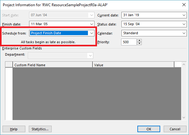
The Mechanics of Backward Scheduling
When specified for the active project, this mode essentially does the following:
- Sets the default constraint type for all new tasks to as late as possible (ALAP).
- Re-sets the constraint type to ALAP for all existing Summary tasks.
- [Users choosing this mode in the middle of schedule development must manually re-set the constraint type to ALAP for all existing non-Summary tasks.]
- Automatically sets no later than constraints when dates are manually entered into the start or finish fields of tasks. [Such date entry in forward scheduling mode leads to “no earlier than” constraints, so users choosing this mode in the middle of schedule development should manually review, validate, and potentially re-set any previously-entered date constraints.]
- Performs the network scheduling calculations in reverse order, with the reflection point occurring at the project start rather than the project finish. I.e. the project start date (not the finish, which is user-input) is determined by the logic.
- Sets the start and finish of automatically-scheduled tasks to their late dates rather than their early dates. (This is the most important part.)
- Finally, the resource leveling engine resolves resource over-allocations by accelerating higher priority tasks from late dates rather than delaying lower priority tasks from early dates. Thus, entries in the leveling delay field are negative. This behavior creates a minor complication regarding use of priority = 1000. Just as in forward scheduling, a task with priority=1000 is always exempted from any leveling action. In backward scheduling, this means that priority values of 1000 and 0 are essentially equivalent when considered in the leveling decisions. The highest effective priority for controlling leveling behavior then becomes 999, not 1000.
Logic relationships used in backward scheduling still have exactly the same meanings that they do in forward scheduling. A finish-to-start (FS) relationship still means that the two tasks are logically connected such that the successor may not start before the predecessor finishes, and the rarely-applicable start-to-finish (SF) relationship still indicates that it is impossible for the successor to finish before the predecessor starts. Some users seem to think that backward scheduling involves reversal of these two relationships in particular, but that’s not consistent with the rest of the backward scheduling mode. Unfortunately, mixing of the two approaches seems to continue, though this typically amounts to invalid date manipulation in my view.
In normal (i.e. forward) scheduling, a task with an ALAP constraint has the dubious distinction of corrupting its entire chain of successors – driving all of them to the critical path. There are very few legitimate applications for this constraint. In backward scheduling, the as soon as possible (ASAP) constraint plays a similar role, corrupting its chain of predecessors. It needs to be avoided in backward scheduling.
When to Use Backward Scheduling
I’ve never used backward scheduling in a real project. Others have recommended its use to determine the desired start date of a project when the desired completion date is already known. It also seems consistent, when tasks are suitably buffered, with aspects of critical chain project management that require work to be scheduled as late as possible.
Ultimately, backward scheduling rests on the presumption that tasks can be accelerated (i.e. moved to the left on the bar chart) indefinitely as needed to meet the fixed end date for the project. Thus, a task whose duration is extended can simply be re-scheduled to start sooner than previously planned, with its predecessors also being accelerated. Similarly, a higher priority task can be started (and finished) earlier to avoid resource conflicts with a lower-priority task that demands the same resources. The problem with these presumptions is that time invariably marches forward, and as scheduled dates for incomplete work are overtaken by the vertical time-now line on the bar chart there is no chance for recovery. The backward scheduling method is pointless if the latest allowable project start date has already been passed – e.g. the project is in progress.
Backward scheduling seems to be of primary value in determining the latest responsible date to start a project (or project segment) while still meeting the desired completion date. After that latest responsible start date is determined, the project must be converted from backward-scheduled to forward-scheduled mode – manually reviewing and revising the key parameters of each task – if it is to be used for updating and forecasting during project execution. The original question – i.e. what is the latest responsible project start date? – is just as easily answered by manipulating and examining the late dates of the forward scheduled project. Thus, for a competent project scheduler, the use of backward scheduling seems largely to be an unproductive diversion.
Driving Logic Analysis
When the logic network is well constructed – and complicating factors like multiple calendars, (early) constraints, and resource leveling are avoided – then the critical path may be reasonably identified by total slack = 0. Other methods of driving logic analysis must be modified, however.
Under backward scheduling, any slack/float of a task exists on the side towards its predecessors, i.e. to its left on a bar chart. A driving relationship exists when a successor prevents a predecessor from being scheduled any later than it is. This means that there are driving successors and driven predecessors. Consequently, the Longest Path in a backward scheduled project is the driving (successor) path from the project’s start.
MSP includes two built-in methods for reviewing and analyzing driving logic: the Task Inspector pane and the task paths bar styles. As I wrote in this article a few years ago, I’ve found these tools to be unreliable in complex real-world project schedules. Under backward scheduling, they are essentially useless and/or misleading.
To start with, Task Inspector simply doesn’t work with backward scheduling. Opening TI on a backward scheduled project yields the following message: This project is set to Schedule from Finish. We are unable to provide scheduling information.
Also under backward scheduling, the Driving Predecessors and Driven Successors bar styles are still derived from Early Dates, as they are in Forward Scheduling. This makes them essentially useless for assessing the controlling logic of the displayed (late-dates) schedule. Consider the example below, where all four Task Path bar styles have been imposed, and Task 11 – A2 Structures – is selected. (The automatic “Slack” bar style is also imposed, but it is invisible since Free Slack – formally defined by Early dates alone – is uniformly zero.) 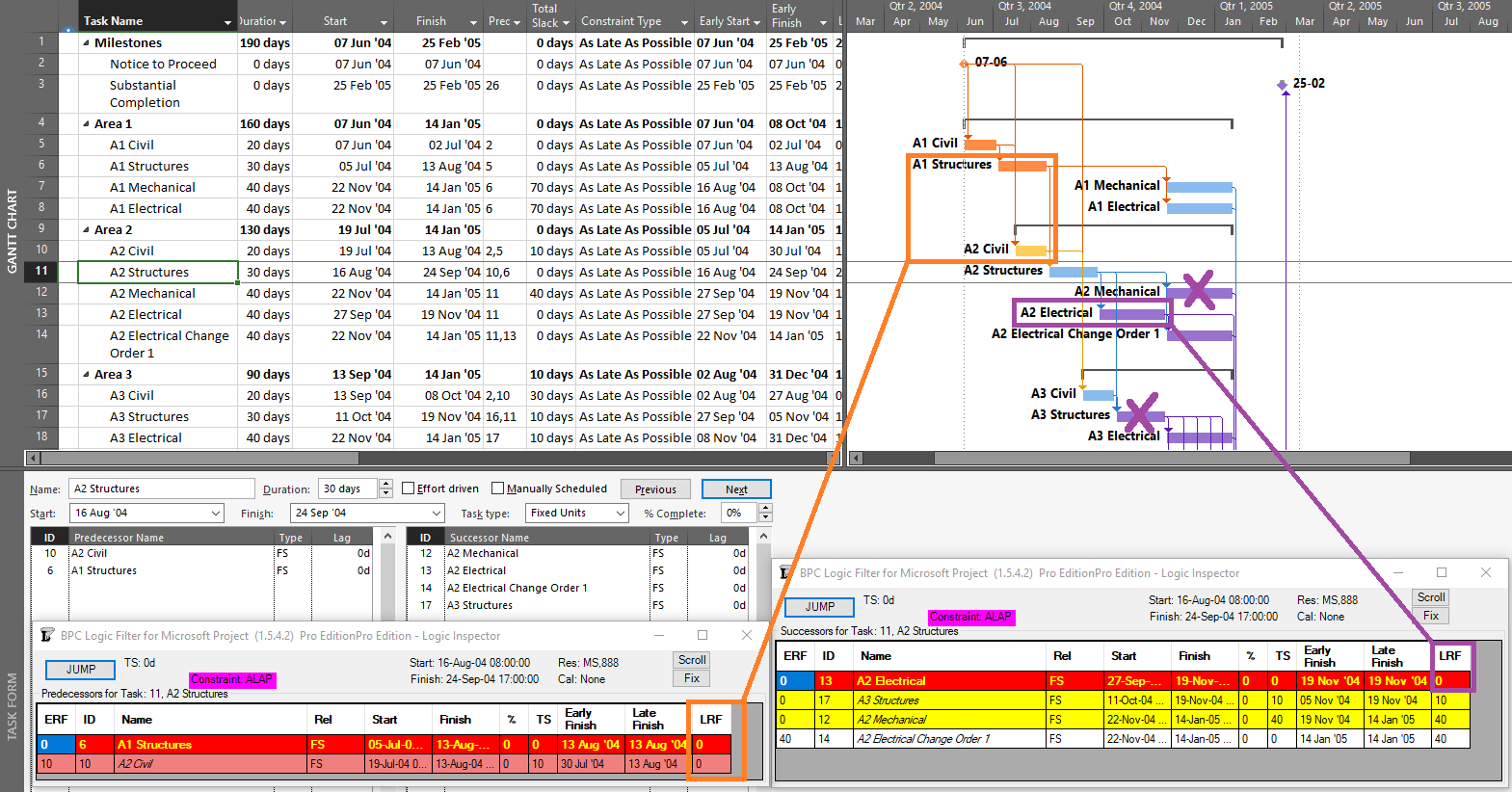
The selected task is in fact driving/controlling the displayed dates of both of its predecessors (LRF=0), but only one of them displays the correct bar style (the one that, with ERF=0, was the driving predecessor during the forward pass). Of Task 11’s four successors, only the first (Task 13 – A2 Electrical) is directly driving/controlling Task 11’s schedule, with LRF=0. The tasks for two of the remaining three successor relationships are incorrectly highlighted, while the third (Task 14) is correctly highlighted only because it is driving/controlling Task 13 – a case of redundant logic. (All four successors were driven successors during the forward pass.) Thus in a backward scheduled project, the Task Path bar styles for Driving and Driven dependencies are meaningful (or “correct”) ONLY along the Longest/Critical path of the project, where Early dates and Late dates coincide. The relationships along that path are driving in both directions; i.e. they are bi-directional driving relationships.
BPC Logic Filter – my company’s Add-In for logic analysis of MSP schedules – identifies driving logic based on relationship free float, which we often call “relative float.” In BPC Logic Filter, the Longest Path and near-longest paths of simple, backward-scheduled projects can be found using the Task Logic Tracer, starting from the project start milestone and using appropriate settings (i.e. driving relationships in successor direction). As illustrated in the example project, this is fairly trivial since the results are 100% aligned with Total Slack. 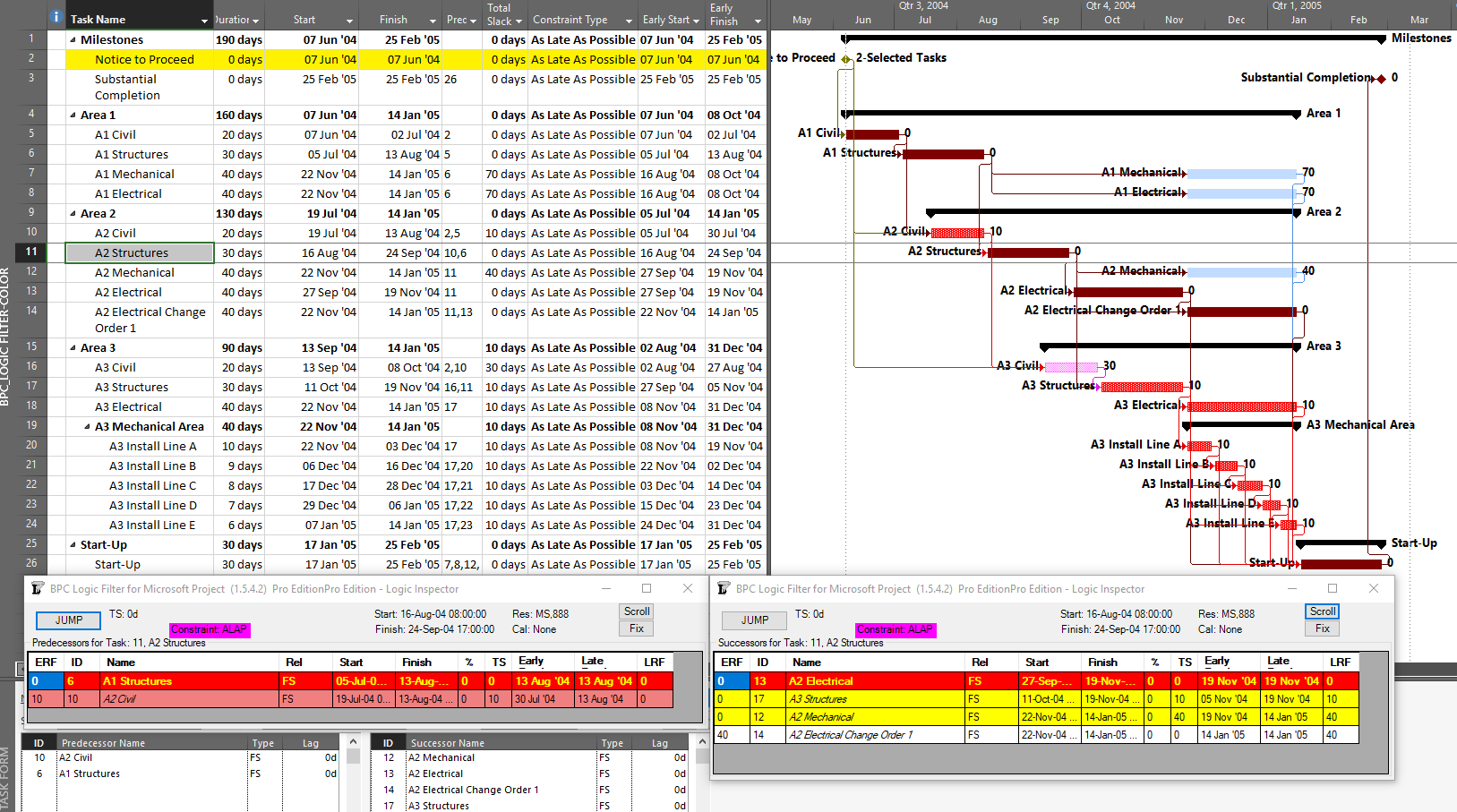
Other driving logic paths (not on the Critical Path) are not so trivial but are easily addressed using BPC Logic Filter, provided that the impact of multiple calendars is minimal.
Precision analysis of more complex, backward-scheduled projects requires some modest modifications to the algorithms. In particular, several variations of late-relationship-float need to be computed, and these have been added to the development roadmap for the software.
[Apr’20 Revision. I’ve updated the two figures to incorporate the early-date relative float (ERF) and late-date relative float (LRF) columns in the logic inspector windows. Calculation of the latter was only added to recent builds of BPC Logic Filter. These windows also flag the forward-driving (yellow), backward-driving (rose), and bi-directional-driving (red/yellow) relationships.]