BPC Logic Filter – TomsBlog

Video – Inspect and Jump through Network Logic Links Using BPC Logic Filter – LLI Edition

Here’s a video of the new Limited Logic Inspector (LLI) in action. The LLI Edition of BPC Logic Filter is for those MS Project users looking to examine the schedule logic network, but without a need for advanced analysis or reporting of logic flow. It’s pretty smooth.

Multiple Critical Paths – Revisited with BPC Logic Filter

While writing an article on Multiple Critical Paths a few years ago, I knew that BPC Logic Filter (our add-in for Microsoft Project) could easily identify multiple critical paths (and near-critical paths) in any project schedule, but we needed to analyze key milestones one at a time. In most cases I think that’s still the best approach to understanding the factors that drive (and may delay) key project deliverables. Nevertheless, the latest build of the software (1.5.5.13) includes a new setting that facilitates simultaneous analysis and display of the critical paths to multiple milestones in a project or program schedule.

The setting – Group Results by Selected Task – is found on the Tracing Preferences tab of the software settings, and we enabled it as part of the initial distribution of the build. We hope that at least a couple users have been pleasantly surprised.

This short article provides a couple illustrations of the feature in action.

First, here is the simple example project from the previous article. The project comprises six “phases” of inter-related tasks in a Microsoft Project schedule, now displayed using MSP 2016 rather than MSP 2010 as before. The project has no deadlines or constraints, and MSP designates critical tasks (red bars in the chart) based on total slack (TS<=0).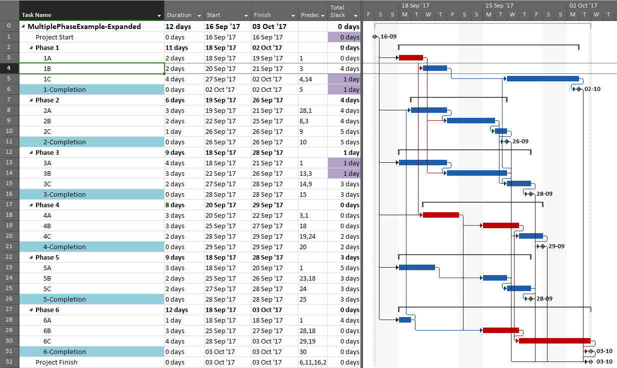

In the previous article, I illustrated – using MSP and Oracle P6 – several generic techniques to identify the unique critical path for each of the six phase completion milestone in the project. I also used BPC Logic Filter to graphically illustrate the critical- and near-critical paths for the Phase 1 completion milestone, displayed within the context of the overall project (and repeated here in MSP 2016).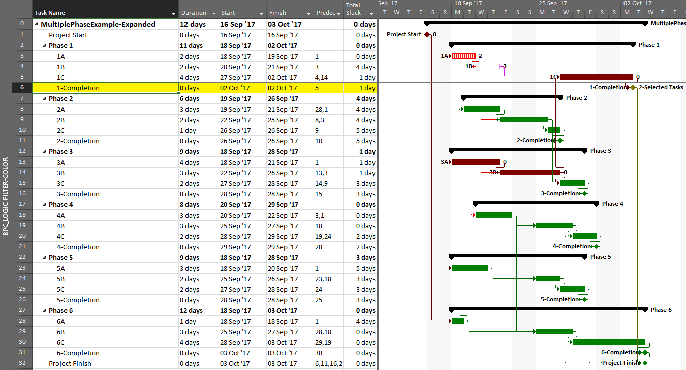

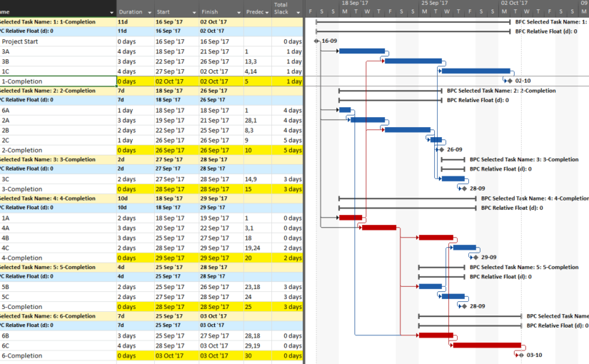
Going back to the original project, we can now run the task logic tracer with all six phase-completion milestones selected. The Standard Edition of BPC Logic Filter then allows us to select driving-path predecessors and to re-sort the results to show logical branches (i.e. paths).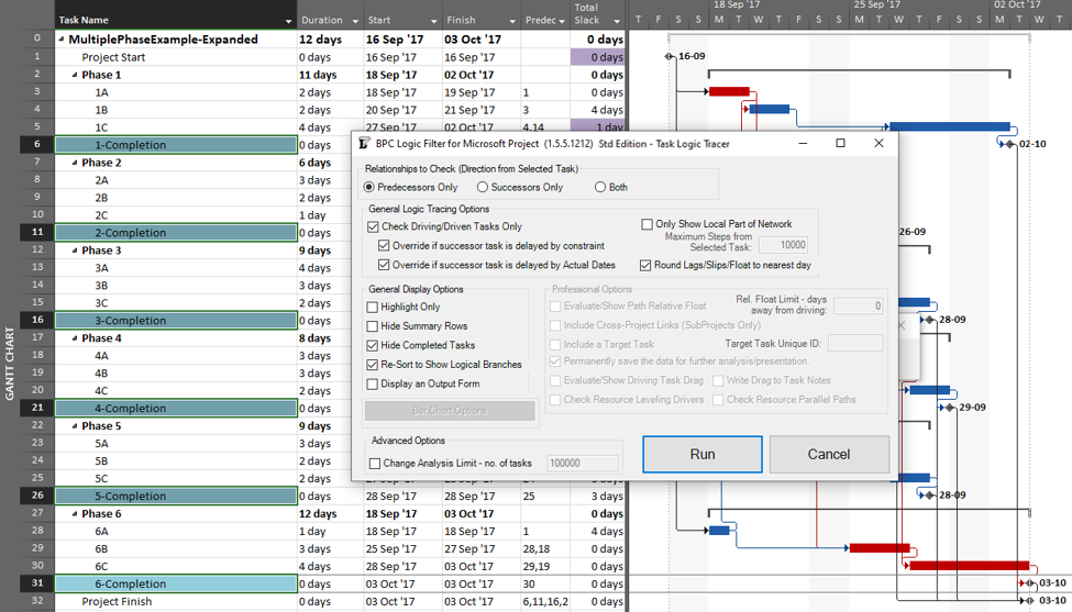

The result is a grouped view displaying the driving predecessor path to each of the six phase-completion milestones.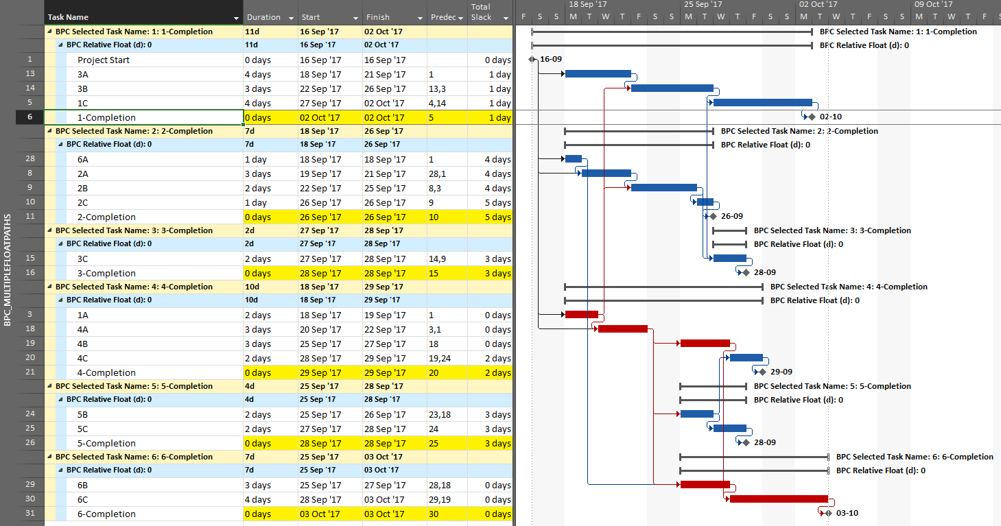

Due to intersecting logic, some tasks are on the driving/critical path for more than one completion milestone, but the Gantt chart only allows them to be displayed once. The task logic tracer displays such tasks together with the driven milestone that is encountered first in the original task selection. Thus, while tasks 1A, 4A, and 4B are critical for the overall project and for the phase-6 completion, they are displayed with the phase 4 completion milestone – for which they are also driving/critical – because that milestone was encountered first in the user’s selection. As a consequence, re-sorting the tasks in the overall project can alter the apparent driving paths for key delivery milestones when intersecting logic is present.

The same caveat applies when considering near-driving/critical paths for multiple key milestones in the same project, along with an added condition that a non-driving task will be included with whichever key milestone it is nearest to driving. To illustrate, we have re-run the previous analysis while considering path relative float, and we’ve decided to re-color bars to clarify results.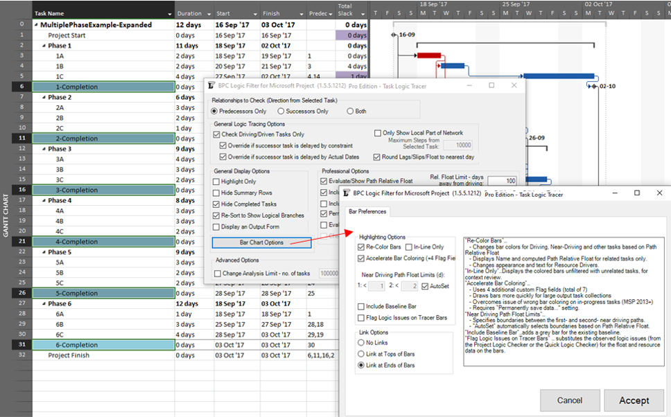

The resulting output is like the earlier one, but now including annotated bars and tasks whose path relative float is above zero (i.e. non-driving).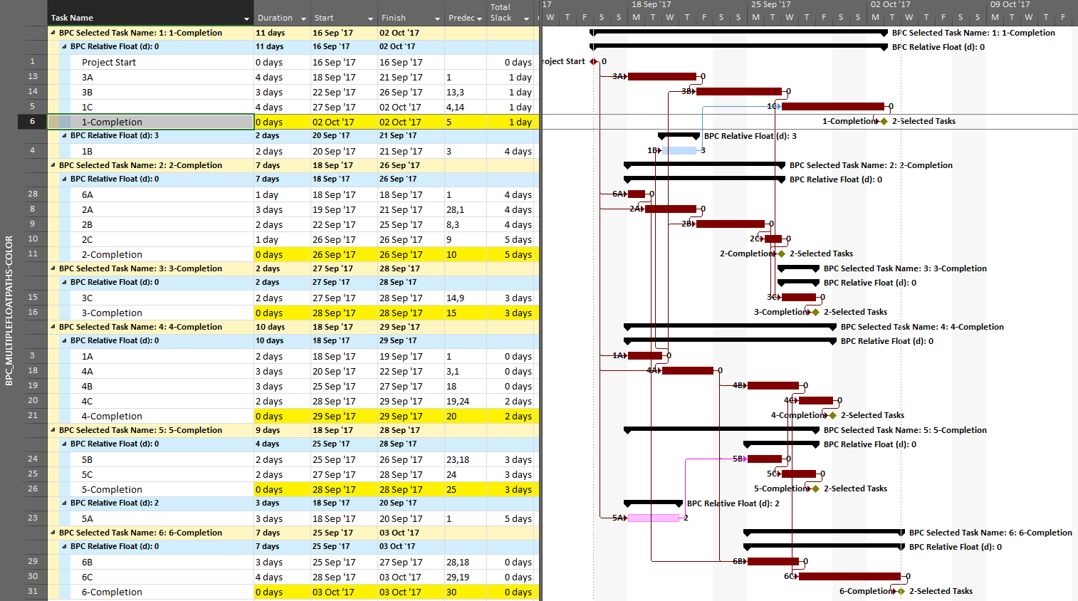

From the earlier article, we already know that task 1A is a non-driving path predecessor of the phase-1 completion milestone, 2 days from driving that milestone. It is nearer to driving (and is in fact driving) the phase-4 completion, however, so that is where it is shown.

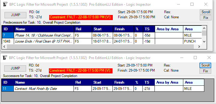
As we’ve seen, it can be difficult to differentiate the critical paths to multiple completion milestones in a complex project with lots of intersecting logic paths. When a project or program includes multiple completion phases that are not closely related, however, the output is straightforward. A good example of this case occurs when multiple unrelated subprojects are combined into a linked master project for reporting purposes. Here I’ve used the New Window dialog to temporarily combine three simple projects into a temporary master. Then I have applied a filter to show only the key completion milestones for the three subprojects. Finally. I’ve run the task logic tracer with all the visible tasks selected. A Pro Edition of the tool is required to analyze linked subprojects, and I’ve limited the relative float analysis to keep the resulting output small.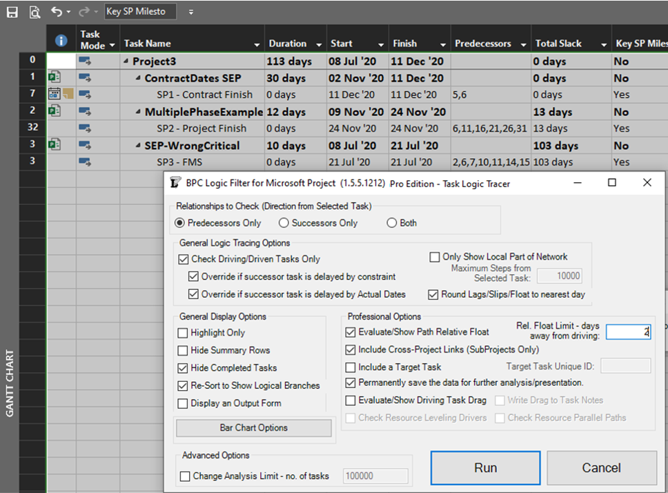

The resulting layout clearly depicts the critical/driving- and near-critical/driving paths for each subproject completion milestone. As usual – for BPC Logic Filter – the definitions of critical/driving logic paths do not rely on the total slack, which is not reliable in many modern project schedules.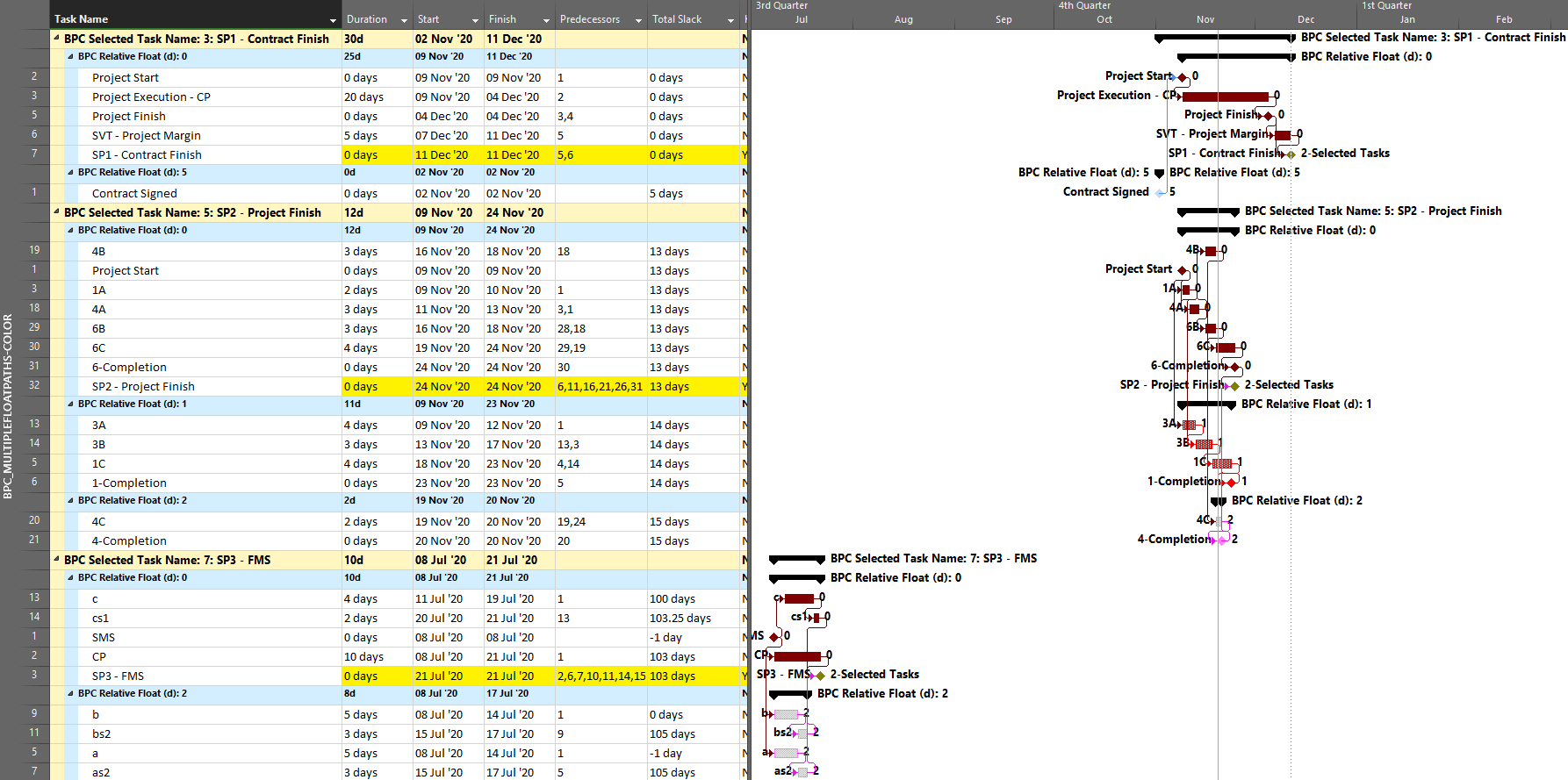

Alternate Definitions of Driving Logic Relationships in Project Schedules

[Article 2 of 2.] This is a summary of the alternate definitions and uses of driving logic relationships between activities in project schedules, as applied in Primavera P6 and Microsoft Project software. Driving relationships are often considered fundamental elements of the project critical path.

This winter I worked with a colleague to prepare a paper – Interpreting Logic Paths in Multi-Calendar Project Schedules – for presentation at this year’s AACE International Conference and Expo in ~~Chicago~~ (Covid-19) virtual world. It’s a deep dive into the Multiple Float Path calculation options in Primavera P6 scheduling software. During the technical study, I had a lot of opportunities to think about driving logic relationships. I’ve summarized the standard definitions and uses in an earlier article. This entry summarizes the alternate versions of driving logic relationships that sometimes arise.

The Importance of Driving Logic

The planning and execution of complex projects requires the project team to understand, implement, and communicate the consequences of schedule logic flow to the other stakeholders. Through schedule logic, each activity in the project has the potential to constrain or disrupt numerous other activities – and to be constrained or disrupted by them. The most obvious artifacts of logic flow are the important logic paths, like the critical path, the Longest Path (in Primavera P6), or the driving path to a key delivery milestone. Regardless of the detailed definition, each of these important paths is governed by driving logic relationships from the first activity to the last activity in the path.

Late-Dates and Bi-Directional Driving Relationships in Primavera P6

From the earlier article, a relationship is considered driving (under the standard definitions) when its successor’s early dates are constrained by the relationship, during the forward pass of the CPM calculations. That is, standard driving relationships are early-dates driving relationships. A late-dates driving relationship, in contrast, is one that constrains the late dates of the predecessor, during the backward pass. When an activity has multiple successors, then one or more of these successor relationships may be controlling the late dates, and hence the total float, of the selected activity; this is a late-dates driving relationship.

Identification of late-dates driving relationships is a key factor in P6’s Multiple Float Path (MFP) calculation. Under the total float calculation option, a relationship can be assigned to a driving “float path” only if it meets the criteria for both early-dates and late-dates driving relationships. That is, it possesses bi-directional driving logic. Since P6 does not flag or otherwise mark such relationships, the results of multiple float path calculations with the total float option can be confusing. Full understanding of the float paths may require a detailed examination of relationship and activity floats, especially when multiple calendars or constraints are involved.

For more information on MFP calculations in P6, check out these other entries in the blog:

Beyond the Critical Path – the Need for Logic Analysis of Project Schedules

P6 Multiple Float Path Analysis – Why Use Free Float Option

Relationship Free Float and Float Paths in Multi-Calendar Projects (P6 MFP Free Float Option)

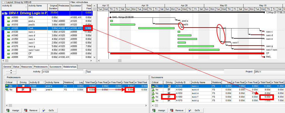
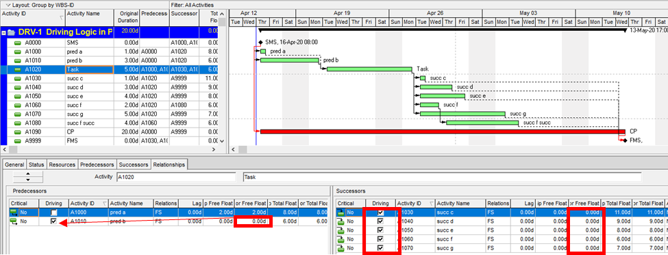
Aside from the MFP calculation option in P6, this type of driving logic is useful mainly for prioritizing driving successors when click-tracing through the schedule network in the forward direction – perhaps for schedule validation or disruption analysis. For example, consider the selected activity (A1020, “Task”) in the P6 version of our simple project below. A glance at the late-date bars shows that only one of its five driven successors (A1060, “succ f”) is responsible for the late dates (and total float) of the selected task. The corresponding relationship possesses bi-directional driving logic and marks the forward continuation of the total-float-based driving path. In the relationship tables, the “Driving” checkboxes already indicate the relationships with early-dates driving logic. When exploring forward, most P6 users will simply click to the driven successor activity that is “Critical” or has the lowest total float value, and that will be correct much of the time. When multiple constraints and/or calendars exist, however – or when the path being explored is far from critical – then late-dates driving logic is indicated when the “Relationship Total Float” equals the total float of the predecessor activity, as highlighted in the figure.

Late-Dates and Bi-Directional Driving Relationships in BPC Logic Filter

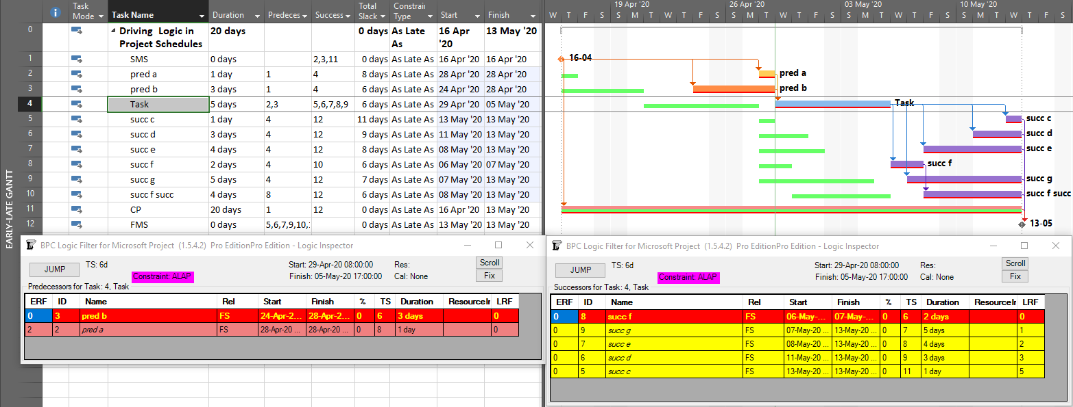
With no built-in alternatives, BPC Logic Filter automatically identify all three types of driving relationships – early-dates, late-dates, and bi-directional – in Microsoft Project schedules. The next figure repeats the same simple example project from the earlier article, with additional bars for early and late dates (green and red) and the task paths shown earlier (orange, gold, purple.) Within the logic inspector tables, bi-directional driving relationships are highlighted (red/yellow) and shown on top. Among those relationships that are NOT bi-directional drivers, early-date drivers are shown in the same yellow as before, and late-date drivers are shown in pale red. As usual, the logic inspector’s jump buttons make for easy, logic-based navigation through the schedule.

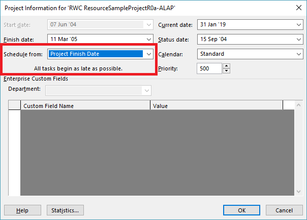
Unlike MSP’s built-in task path bar styles, the logic inspector tables are equally effective at illustrating driving logic in backward-scheduled projects. This is demonstrated below, where the same example project has been re-configured to Schedule from: Project Finish Date. Interestingly, while the scheduled dates clearly change, the nature of driving logic relationships does not.

For further information on driving logic in backward-scheduled projects, check out this earlier entry: Driving Logic in Backward Scheduled Projects (Microsoft Project), which pre-dated the introduction of late-dates driving calculations in the logic inspector.

Resource Driving Logic Relationships in BPC Logic Filter

When resource leveling is imposed in a P6 or MSP project schedule, some tasks are delayed from their CPM-based early dates until resources become available – after completion of other tasks. In the figure below, a single resource has been assigned to the five successors of the “Task,” and the resulting overallocation of the resource has been resolved by leveling the schedule using the simplest options. As a result, the project finish milestone has been delayed by three days, and the critical path has shifted.

The leveling process creates implied driving relationships between tasks that demand the same resources. BPC Logic Filter infers these “ResDrvr” relationships. As shown below, the resulting resource-constrained driving logic paths are typically very different from those identified using CPM logic alone.

The consequences of resource driving logic are further addressed in these earlier articles:

Resource Leveling Breaks the “Critical Path” – Logic Analysis of Resource-Leveled Schedules (MS Project)

The Resource Critical Path – Logic Analysis of Resource-Leveled Schedules (MS Project), Part 2

Hierarchical (Parent-Child) Driving Logic Relationships in Microsoft Project

Unlike other project scheduling tools, MSP supports direct assignment of schedule logic (start predecessors and finish successors only) to “summary tasks.” As a consequence, it then imposes automatic logic restraints based on the relative positions of tasks within the Outline/Work breakdown structure. Thus, a summary task with a finish-to-start predecessor automatically imposes a corresponding early-start restraint on every one of its subtasks, and this restraint is inherited at each outline level all the way to the lowest-level subtask. Moreover, a summary task with a finish to start successor automatically imposes a corresponding late-finish (backward-pass) restraint on its subtasks, which is inherited all the way down the outline structure. External date constraints, manual-mode scheduled dates, and actual dates inputs for summary tasks have similar consequences.

The immediate early-start drivers for summary tasks and subtasks – whether a result of predecessor logic, outline-parent inheritance, or outline-child roll-up – can be identified by the task Inspector as shown in the next figure, and some of these are explicitly enumerated in the “driver” collections of the task. The late-date consequences remain implicit, however.

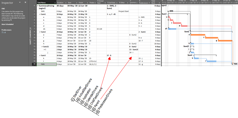
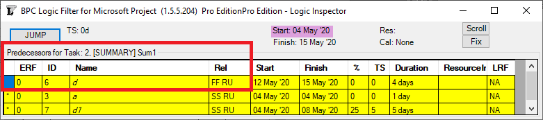
The apparent critical path for the schedule of the previous figure runs through tasks a-d and tasks e-g, including their driving FS relationships. Not shown, however, is the implicit driving FF relationship from task d to its outline parent task Sum1 (here identified in BPC’s logic inspector tool.)

The implicit driving SS relationship from task Sum2 to its outline child task e is correctly identified by the task inspector as well as BPC’s logic inspector.

Those two implicit hierarchical relationships – when combined with the explicit Sum1-to-Sum2 FS relationship – are necessary to properly calculate early and late dates and total slack, which is the source of the critical path depicted. Unfortunately, the built-in tools are not sufficient to fully trace driving logic through such hierarchical relationships, even in this simple schedule.

Neither summary-task relationships nor the consequent hierarchical (parent/child – child/parent) relationships are explicitly recognized in the generally accepted, traditional understandings of logic-based project scheduling – i.e. the critical path method (CPM) and the precedence diagramming method (PDM). Such relationships are not generally supported in other scheduling tools, either, so attempts to migrate MSP schedules containing summary logic into other tools for analysis are typically unsuccessful. It is also clear that adding even a small number of summary-task relationships to a moderately complex project schedule can potentially obfuscate the driving logic paths in the schedule, including the critical path under many circumstances, without fairly sophisticated analysis. Taking these facts together, most project scheduling professionals seem to agree that summary-task logic in MSP represents poor practice and is to be avoided.

Driving Logic Relationships in Project Schedules

[Article 1 of 2.] This is a summary of the standard definitions and uses of driving logic relationships between activities in project schedules, as applied in Primavera P6 and Microsoft Project software. Driving relationships are often considered fundamental elements of the project critical path.

This winter I worked with a colleague to prepare a paper – Interpreting Logic Paths in Multi-Calendar Project Schedules – for presentation at this year’s AACE International Conference and Expo in ~~Chicago~~ (Covid-19) virtual world. The paper reflects a deep dive into the Multiple Float Path calculation options in Primavera P6 scheduling software. During the technical study, I had a lot of opportunities to think about driving logic relationships. This entry summarizes the standard definitions and uses. I’ve summarized a couple alternate definitions and uses in another article.

The Importance of Driving Logic

Standard Definition and Uses of Driving Logic Relationships

A driving relationship is “A relationship between two activities in which the start or completion of the predecessor activity determines the early dates for the successor activity with multiple predecessors. See also: Free Float.” [That’s the standard definition from AACE International.] Alternately, “A driving relationship is one that controls the start or finish of a successor activity.” [That’s from the PMI publication on CPM Scheduling for Construction.]

For practical purposes, a driving relationship is a predecessor relationship that prevents a successor activity’s early start or early finish from being scheduled any earlier than it is. When an otherwise unconstrained activity has only one predecessor, then it is normally, and obviously, a driving predecessor. When an activity has multiple predecessors, then one or more of them may be driving while the others are non-driving. These distinctions answer the key questions, “Why is this activity scheduled when it is? Why can’t we do it sooner?”

Driving Logic in Primavera P6

Like its predecessors, P6 routinely illustrates driving logic relationships using solid lines on bar charts – either red or black depending on the “Critical” status of the connected activities. Non-driving relationships are depicted with the same colors, and those that are also non-critical use dotted lines. This is demonstrated in the figure below, where the non-critical activity “Task” (A1020) has two predecessors and five successors. One of the predecessor relationships and all five of the successor relationships are depicted with solid black lines and marked as driving (but not critical) in the relationship tables. The non-driving relationships – one from “pred a” to “Task” and five more from Task’s successors to the project’s finish milestone – are depicted with dotted lines. The two critical, driving relationships that connect the “CP” activity to the project’s start and finish milestones are depicted with solid red lines.

In small projects it is often easy to identify driving logic flow in printed P6 bar charts by visually tracing the solid relationship lines between activities. As project schedules become larger and more complex, however, the number of relationship lines increases to the point that visual tracing becomes impractical. Then driving relationships are primarily identified using the relevant columns of the associated relationship tables. Experienced P6 users often use the “GoTo” buttons in the relationship tables to click-trace along driving logic paths – backward and forward through complex project schedules – to review and confirm important chains of sequential logic (i.e. driving logic paths).

In general, Primavera P6 identifies driving relationships by analyzing the intervals between early dates of the linked activities, after completion of the core scheduling calculations. With a few minor exceptions, a driving relationship is identified when the Relationship Successor Free Float (RSFF) equals zero. In addition to providing a basis for the graphical and tabular depictions of driving logic flow, P6 uses these driving attributes to automatically identify the Longest Path, or the driving path to project completion.

Driving Logic in Microsoft Project

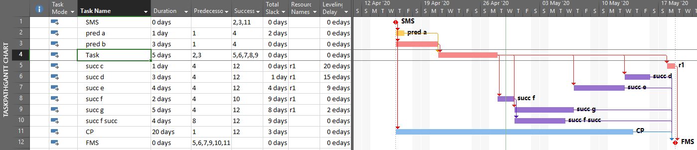
Unlike P6, Microsoft Project (MSP) does not graphically differentiate driving and non-driving relationship lines in Gantt-chart views, and the standard relationship (i.e. dependency) tables provide no driving-logic indicators. The Task Inspector pane provides the primary method for identifying driving predecessors of the currently-selected task; there is no corresponding method for identifying driven successors. The figure below depicts the same schedule as before, now in MSP format, with the Inspector pane identifying a single (driving) predecessor task, “pred b”, for the currently-selected task (“Task.”) As far as it goes, this agrees with P6.

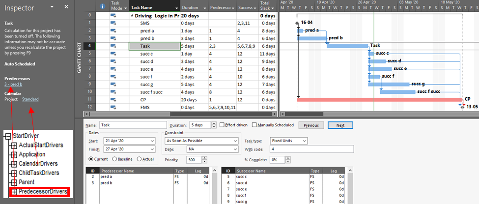
Although not presented to users, driving relationship indicators are developed by MSP (at least since MSP 2007), with the results being stored in the PredecessorDrivers collection for each task. This collection forms the basis of the Predecessors list of the Inspector pane.

It’s also apparent that the PredecessorDrivers data are used to define the Driving Predecessors and Driven Successors bar styles that were introduced as part of the Task Path functionality in MSP 2013. This functionality is illustrated below, where the driving and non-driving predecessors of “Task” – and its driven successors – are all differentiated by bar color. Although there are clear limitations to this graphical approach, the ability to show driving and driven logic paths (if not individual driving relationships) is a major improvement for MSP users.

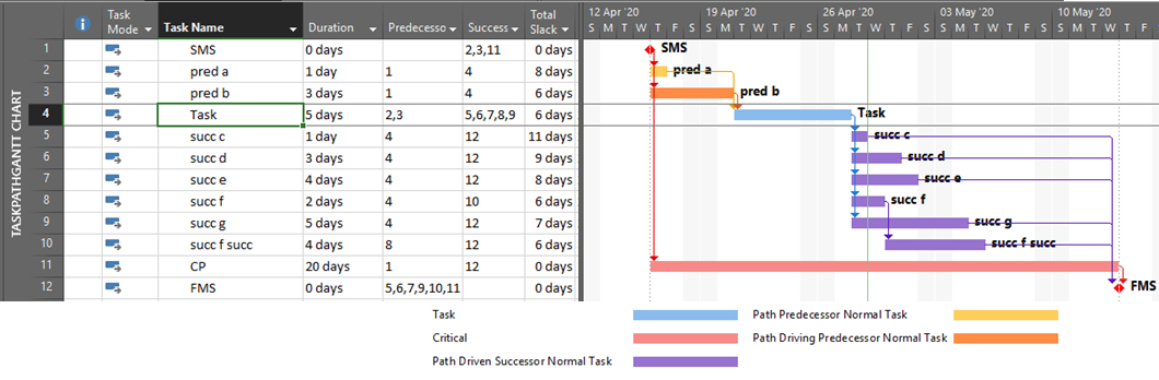
Unfortunately, the internal MSP calculation of driving logic attributes – and the explicit paths of driving logic that they purport to illustrate – have proven unreliable for complex schedules with other than finish-to-start relationships, out-of-sequence progress, or external links.

Standard Driving Logic in BPC Logic Filter for Microsoft Project

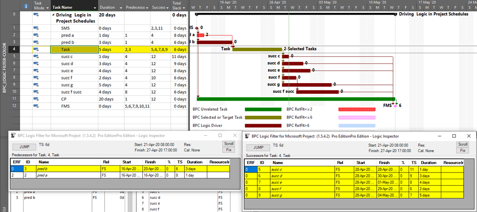
BPC Logic Filter (my company’s add-in for MSP) identifies driving logic by independently analyzing relationship relative floats after completion of the schedule calculations. This is a bit like the P6 approach and has proven, at least for me, more reliable than the internal MSP data when things get complicated. This figure shows the combination of a logic tracer view (with special bar styles depicting driving and near-driving logic paths) together with the task logic inspector tables. Driving relationships are highlighted yellow in the tables. Overall, this seems to combine the best parts of the corresponding P6 and MSP layouts, and the Jump buttons allow for logic-based navigation forward or backward through the schedule network.

Continue to related article…

Alternate Definitions of Driving Logic Relationships in Project Schedules

Construction CPM Conference 2019 – Schedule Logic in Microsoft Project

Click Here to view the screen and audio capture of my presentation (on BPC Logic Filter) at the 2019 Construction CPM Conference. Fred Plotnick (the Conference organizer) is kind enough to host the content on his server.

Most of this will be familiar to those who’ve already seen one of my presentations on BPC Logic Filter, but the questions and answers beginning at about minute 59:00 are new.

Driving Logic in Backward Scheduled Projects (Microsoft Project)

Microsoft Project’s backward scheduling mode includes numerous traps for novices and professionals alike. Competent project schedulers avoid it.

In MSP, a backward scheduling mode – sometimes called backward planning, reverse scheduling, or reverse planning – can be invoked by scheduling the project from its finish rather than its start. In the traditional language of critical path method (CPM) scheduling, it’s most simply described as a late-dates schedule. Backward planning is useful in several non-standard methodologies, including critical chain project management and the pull planning aspects of the Last Planner System.

The Mechanics of Backward Scheduling

When specified for the active project, this mode essentially does the following:

Sets the default constraint type for all new tasks to as late as possible (ALAP).
Re-sets the constraint type to ALAP for all existing Summary tasks.
[Users choosing this mode in the middle of schedule development must manually re-set the constraint type to ALAP for all existing non-Summary tasks.]
Automatically sets no later than constraints when dates are manually entered into the start or finish fields of tasks. [Such date entry in forward scheduling mode leads to “no earlier than” constraints, so users choosing this mode in the middle of schedule development should manually review, validate, and potentially re-set any previously-entered date constraints.]
Performs the network scheduling calculations in reverse order, with the reflection point occurring at the project start rather than the project finish. I.e. the project start date (not the finish, which is user-input) is determined by the logic.
Sets the start and finish of automatically-scheduled tasks to their late dates rather than their early dates. (This is the most important part.)
Finally, the resource leveling engine resolves resource over-allocations by accelerating higher priority tasks from late dates rather than delaying lower priority tasks from early dates. Thus, entries in the leveling delay field are negative. This behavior creates a minor complication regarding use of priority = 1000. Just as in forward scheduling, a task with priority=1000 is always exempted from any leveling action. In backward scheduling, this means that priority values of 1000 and 0 are essentially equivalent when considered in the leveling decisions. The highest effective priority for controlling leveling behavior then becomes 999, not 1000.

Logic relationships used in backward scheduling still have exactly the same meanings that they do in forward scheduling. A finish-to-start (FS) relationship still means that the two tasks are logically connected such that the successor may not start before the predecessor finishes, and the rarely-applicable start-to-finish (SF) relationship still indicates that it is impossible for the successor to finish before the predecessor starts. Some users seem to think that backward scheduling involves reversal of these two relationships in particular, but that’s not consistent with the rest of the backward scheduling mode. Unfortunately, mixing of the two approaches seems to continue, though this typically amounts to invalid date manipulation in my view.

In normal (i.e. forward) scheduling, a task with an ALAP constraint has the dubious distinction of corrupting its entire chain of successors – driving all of them to the critical path. There are very few legitimate applications for this constraint. In backward scheduling, the as soon as possible (ASAP) constraint plays a similar role, corrupting its chain of predecessors. It needs to be avoided in backward scheduling.

When to Use Backward Scheduling

I’ve never used backward scheduling in a real project. Others have recommended its use to determine the desired start date of a project when the desired completion date is already known. It also seems consistent, when tasks are suitably buffered, with aspects of critical chain project management that require work to be scheduled as late as possible.

Ultimately, backward scheduling rests on the presumption that tasks can be accelerated (i.e. moved to the left on the bar chart) indefinitely as needed to meet the fixed end date for the project. Thus, a task whose duration is extended can simply be re-scheduled to start sooner than previously planned, with its predecessors also being accelerated. Similarly, a higher priority task can be started (and finished) earlier to avoid resource conflicts with a lower-priority task that demands the same resources. The problem with these presumptions is that time invariably marches forward, and as scheduled dates for incomplete work are overtaken by the vertical time-now line on the bar chart there is no chance for recovery. The backward scheduling method is pointless if the latest allowable project start date has already been passed – e.g. the project is in progress.

Backward scheduling seems to be of primary value in determining the latest responsible date to start a project (or project segment) while still meeting the desired completion date. After that latest responsible start date is determined, the project must be converted from backward-scheduled to forward-scheduled mode – manually reviewing and revising the key parameters of each task – if it is to be used for updating and forecasting during project execution. The original question – i.e. what is the latest responsible project start date? – is just as easily answered by manipulating and examining the late dates of the forward scheduled project. Thus, for a competent project scheduler, the use of backward scheduling seems largely to be an unproductive diversion.

Driving Logic Analysis

When the logic network is well constructed – and complicating factors like multiple calendars, (early) constraints, and resource leveling are avoided – then the critical path may be reasonably identified by total slack = 0. Other methods of driving logic analysis must be modified, however.

Under backward scheduling, any slack/float of a task exists on the side towards its predecessors, i.e. to its left on a bar chart. A driving relationship exists when a successor prevents a predecessor from being scheduled any later than it is. This means that there are driving successors and driven predecessors. Consequently, the Longest Path in a backward scheduled project is the driving (successor) path from the project’s start.

MSP includes two built-in methods for reviewing and analyzing driving logic: the Task Inspector pane and the task paths bar styles. As I wrote in this article a few years ago, I’ve found these tools to be unreliable in complex real-world project schedules. Under backward scheduling, they are essentially useless and/or misleading.

To start with, Task Inspector simply doesn’t work with backward scheduling. Opening TI on a backward scheduled project yields the following message: This project is set to Schedule from Finish. We are unable to provide scheduling information.

Also under backward scheduling, the Driving Predecessors and Driven Successors bar styles are still derived from Early Dates, as they are in Forward Scheduling. This makes them essentially useless for assessing the controlling logic of the displayed (late-dates) schedule. Consider the example below, where all four Task Path bar styles have been imposed, and Task 11 – A2 Structures – is selected. (The automatic “Slack” bar style is also imposed, but it is invisible since Free Slack – formally defined by Early dates alone – is uniformly zero.)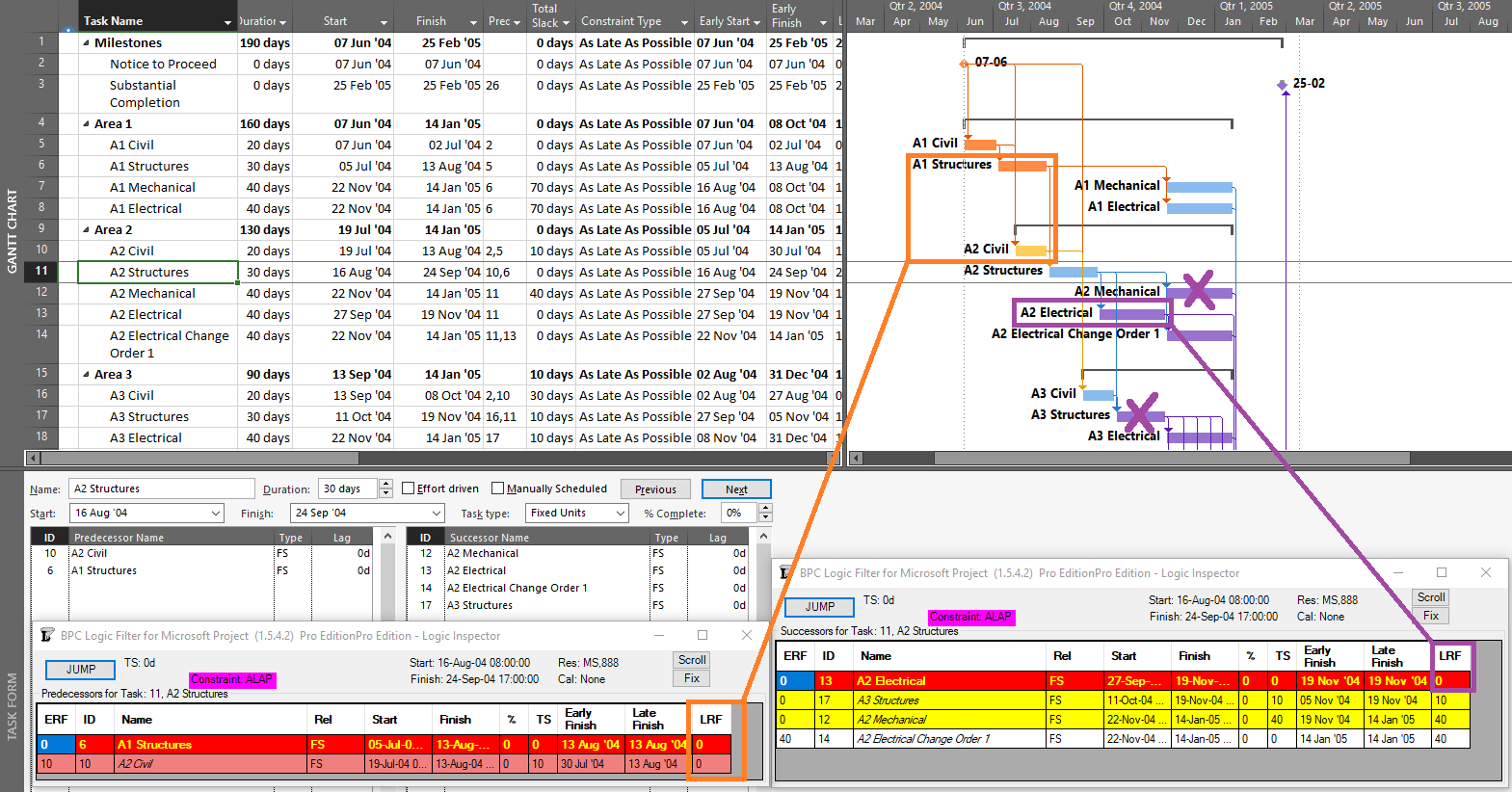

The selected task is in fact driving/controlling the displayed dates of both of its predecessors (LRF=0), but only one of them displays the correct bar style (the one that, with ERF=0, was the driving predecessor during the forward pass). Of Task 11’s four successors, only the first (Task 13 – A2 Electrical) is directly driving/controlling Task 11’s schedule, with LRF=0. The tasks for two of the remaining three successor relationships are incorrectly highlighted, while the third (Task 14) is correctly highlighted only because it is driving/controlling Task 13 – a case of redundant logic. (All four successors were driven successors during the forward pass.) Thus in a backward scheduled project, the Task Path bar styles for Driving and Driven dependencies are meaningful (or “correct”) ONLY along the Longest/Critical path of the project, where Early dates and Late dates coincide. The relationships along that path are driving in both directions; i.e. they are bi-directional driving relationships.

BPC Logic Filter – my company’s Add-In for logic analysis of MSP schedules – identifies driving logic based on relationship free float, which we often call “relative float.” In BPC Logic Filter, the Longest Path and near-longest paths of simple, backward-scheduled projects can be found using the Task Logic Tracer, starting from the project start milestone and using appropriate settings (i.e. driving relationships in successor direction). As illustrated in the example project, this is fairly trivial since the results are 100% aligned with Total Slack.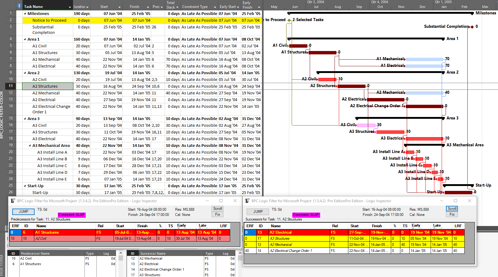

Other driving logic paths (not on the Critical Path) are not so trivial but are easily addressed using BPC Logic Filter, provided that the impact of multiple calendars is minimal.

Precision analysis of more complex, backward-scheduled projects requires some modest modifications to the algorithms. In particular, several variations of late-relationship-float need to be computed, and these have been added to the development roadmap for the software.

[Apr’20 Revision. I’ve updated the two figures to incorporate the early-date relative float (ERF) and late-date relative float (LRF) columns in the logic inspector windows. Calculation of the latter was only added to recent builds of BPC Logic Filter. These windows also flag the forward-driving (yellow), backward-driving (rose), and bi-directional-driving (red/yellow) relationships.]

BPC Logic Filter – Version 1.5 Improvements

The latest release of BPC Logic Filter – an Add-in for schedule logic analysis in Microsoft Project – includes direct implementation of the QuickTrace macros, faster logic-related formatting of Gantt chart bars, additional controls for logic-based schedule navigation, and overall snappier performance.

Introduction

My company started sharing BPC Logic Filter, our Add-in for Microsoft Project, in 2015. Since then, we’ve made incremental improvements to the tool that get shared in real time. Many of these improvements were prompted by informal user feedback, for which we are most grateful. Version 1.5, released in January 2019, brings a few nice little goodies that we’ve been anticipating for a while….

QuickTrace

QuickTrace is a set of macros for simplified logic tracing and filtering in MSP. I wrote the original macros for a blog entry several years ago, and subsequent high traffic on that entry implies that a fair number of MSP users are downloading and implementing the macros. We’ve now partially integrated that code with the rest of the add-in, providing a new ribbon button and a dedicated form, and including QuickTrace in the daily logs.

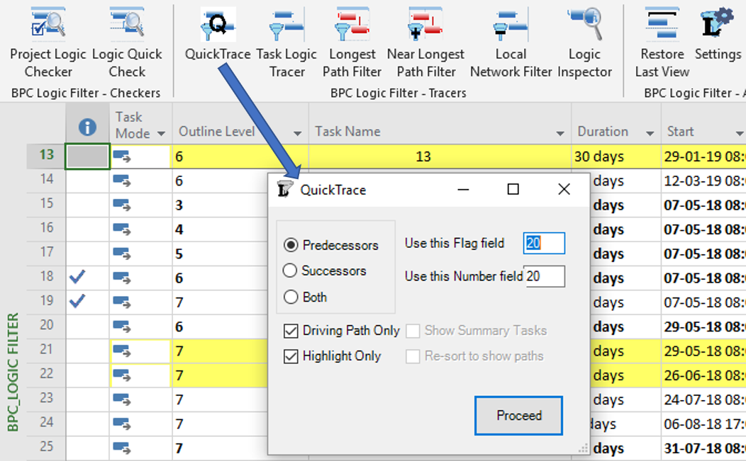
Eventually, we may get rid of the two boxes for selecting custom fields, streamlining the form even more.

QuickTrace is fully aligned with MSP’s internal “Task Inspector” and the associated “Task Path” bar styles (in MSP 2013+). Like the two native tools, QuickTrace relies on internal MSP calculations for identifying “driving” logic. This makes it blazing fast compared to the rest of BPC Logic Filter. Also like the two native tools, it incorrectly identifies driving logic paths in the presence of certain (fairly common) complicating factors.

We’ve included QuickTrace as a reasonable accessory. It is particularly useful when there is a need to compare its results with those of the other logic Tracers in BPC Logic Filter. (This is the chief argument for leaving the QuickTrace custom fields as user-selected, outside the Add-in’s normal routines for selecting and managing its use of custom fields.)

[Because it relies on recursion (a kind of repeated “cloning” of itself), QuickTrace is subject to memory-overload errors. This restricts the maximum path length that can be evaluated before “crashing out.” Based on limited testing, the memory-limited maximum path length (in number of tasks) varies by MSP version and execution environment, as summarized here (figures are approximate).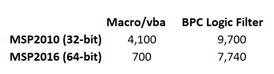

The two obvious conclusions from the table are: 1) MSP 2016 imposes a much larger memory burden than MSP 2010, especially in the nominally-internal vba environment. 2) Compared to the macro/vba, BPC Logic Filter’s implementation of Quicktrace is far less likely to run out of memory on a very large project. This advantage is amplified in MSP 2016. On the downside, the out-of-memory add-in will crash hard, taking your data with it, while the macro/vba solution tends to crash softly.

For the add-in, QuickTrace’s lowest path-length limit – at 7,740 tasks – corresponds to 30 years of 1-day tasks arranged finish-to-start. It seems unlikely that this limit could be reached in a real-world project of at least moderate complexity. Nevertheless, as always, save early and save often.]

Bar Formatting Improvements

The first major upgrade of the tool (v1.1) included the ability to add certain logic-related information to bars in a Gantt Chart, specifically by modifying bar shapes, colors, and text. Such information would be particularly useful for displaying related tasks within the context of an unfiltered view of the overall project schedule (i.e. “In-Line Only”), though I’ve had the habit of re-coloring bars in virtually all analyses.

For several reasons, bar coloring can impose a substantial time penalty on the completion of a logic analysis in BPC Logic Filter, with the size of the penalty being proportional to the number of tasks ultimately displayed. Recent releases of Microsoft Project (e.g. MSP 2013+) have increased the size of this penalty while also introducing some erroneous coloring results for in-progress tasks. Consequently, coloring Gantt bars in very large projects typically has been something to avoid.

Accelerated Bar Coloring

The new “Accelerate Bar Coloring” option is implemented via a single checkbox in the Bar Preferences tab – accessed directly through the “Settings” button on the Ribbon or indirectly through the “Bar Chart Options” button on the control window for each Tracer.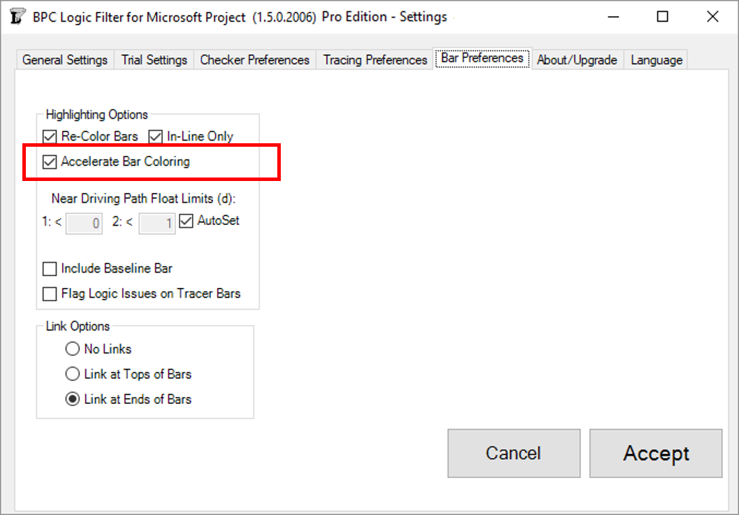

This option introduces an alternate bar coloring process that:

Draws bars more quickly for large filter outputs, with the largest outputs seeing the greatest gain. For example, I have configured a Near-Longest-Path analysis of an 18,000-task schedule to include every task in the output filter. Without bar coloring, the overall analysis takes just under two and a half minutes (145 seconds) on my laptop computer. With Accelerated Bar Coloring, the overall analysis takes 13 seconds more (158 seconds). With traditional bar coloring, the overall analysis takes nearly 20 minutes more!
Overcomes issues of incorrect bar coloring for in-progress tasks (MSP2013+).
Constructs and manages up to 25 new bar styles for uniquely and accurately describing the output. In contrast to the other option, these bar styles can be readily modified and augmented by advanced users of MSP.

These improvements can make the coloring of Gantt bars no longer something to avoid for large project schedules.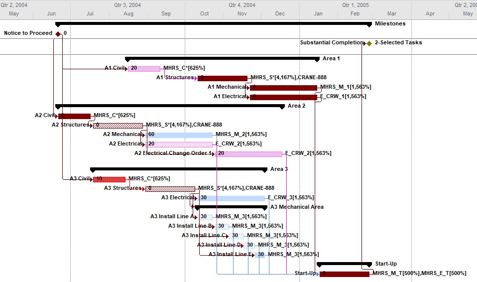

The new option does come at a cost, however. Specifically, it uses 4 more custom Flag fields (in addition to the 3 needed for generating filtered views). Custom fields typically get used up during the execution of a project, and constraining the need for custom fields was one of our key priorities during the early development of BPC Logic Filter. This new demand may force schedulers to be a bit more disciplined in allocating them. The accelerated bar coloring process also has a more rigid requirement for Data Persistence. If “Permanently save the data for further analysis/presentation” is NOT checked, then none of the important information will be shown. (With both the acceleration and permanently-save options turned off, bars are correctly colored, but logic-related text is not shown.) Finally, the additional overhead imposed by the setting can actually slow down the overall analysis and display of a smaller project schedule, so it is not always the fastest.

Link Options

All previous versions of BPC Logic Filter have automatically enforced the inclusion of end-connected link lines (relationship lines) in logic tracing results. The new version leaves this selection to the user.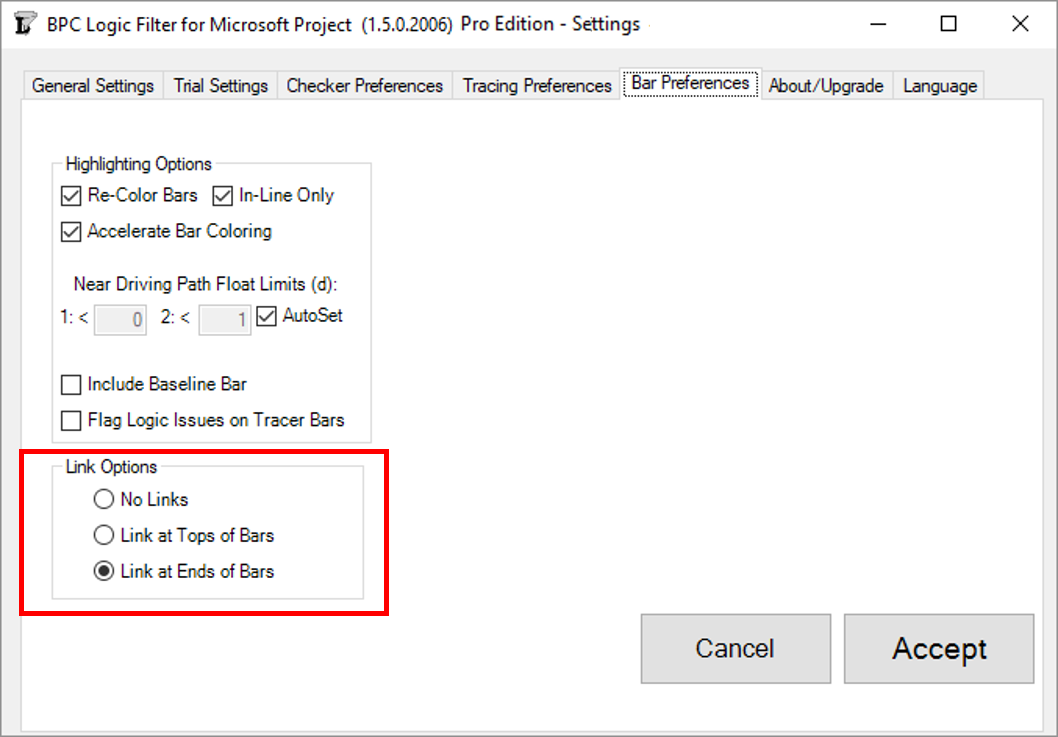

Logic-Jumping Through Hidden Tasks

As any user of MSP’s built-in “Go To” (F5) tool knows, a task must be visible in the existing view to be selected and activated. In the past, this meant that the Logic Inspector Jump buttons – used for navigating through the schedule based on logic relationships alone – could be blocked if portions of the schedule were hidden (by filters or outlining). In the last build of version 1.4, we introduced some features for automatically breaking through such blockages.

Version 1.5 refines and provides for user-control of the behavior. First, it is now possible to fully navigate through any project schedule using the Jump buttons alone, without selecting or activating the tasks in the corresponding task table. This is the behavior demonstrated by the first radio button in the new form below.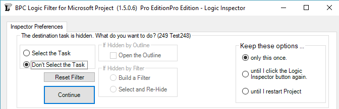

Alternately, the Logic Inspector can automatically select and activate the hidden task by opening a closed Outline (i.e. summary task) where necessary and by adding the task to a temporary filter. (Two types of filter persistence are supported.)

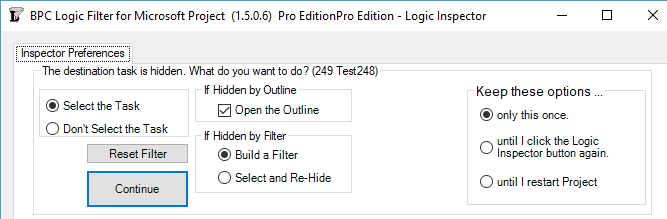
The new form is presented on the first attempt to Jump to a hidden task. The options on the left side of the form tell the software how to handle the specific hidden task. The buttons on the right side tell the software how long to remember this selection. You can always change this decision using the “Reset Filter” button in the Settings.

Streamlined Code and Improved Housekeeping

In addition to the improvements noted above, Version 1.5 incorporates substantial changes to the underlying code base, leading to faster and more efficient analyses.

As a minor note, there is another new user control provided in the General Settings dialog: the “Clear BPC Fields” button. This allows the permanent removal of all BPC-related custom field names and associated data.

Resource Leveling Changes from MSP 2010 to MSP 2016 – Revisited

In a departure from an earlier study, the resource-leveled schedule generated using Microsoft Project (MSP) 2016 may sometimes be substantially shorter than the comparable schedule from MSP 2010. The result suggests a more sophisticated leveling algorithm that, while sometimes generating shorter schedules, may increase the associated resource-related risks.

Several years ago I wrote an article examining some reported differences in resource leveling behavior between Microsoft Project (MSP) 2010 and 2013 versions. In general, those observations implied that the newer software was generating longer schedules under default conditions. (The observations were by others, since at the time I was only using MSP 2010.) I concluded the article with a speculation that the leveling algorithm may have been adjusted to preserve the appearance of the pre-leveling “Critical Path,” but at the expense of a longer schedule.

A recent test case using MSP 2016 does nothing to confirm that speculation, and an opposite conclusion is implied.

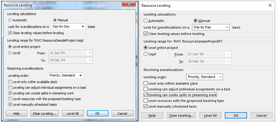
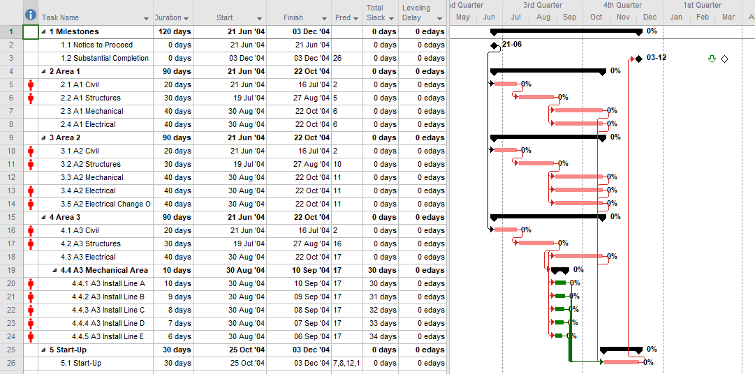
Below is an idealized schedule for construction and commissioning of a small processing plant, including resource loading. Only technologically-required logic is included, so that a) the resources are all severely overallocated, and b) the schedule is unrealistic. The same schedule is shown in both MSP 2010 and MSP 2016 forms, with only cosmetic differences. There is a Deadline of 25Feb’05 on the Substantial Completion task, and no explicit risk buffers are present. [The MSP 2010 form was used to illustrate the resource-leveled critical path in a technical paper I presented at AACE International in 2017.]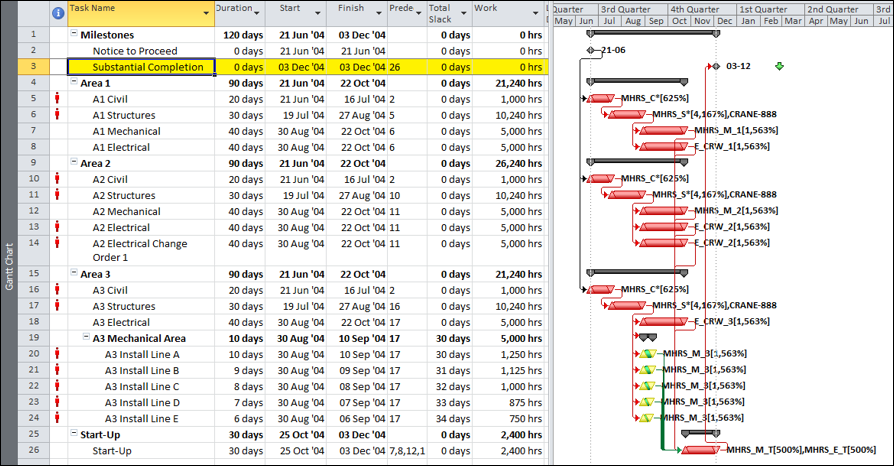

To resolve the resource over-allocations and generate a more realistic schedule, the resource leveler is applied in both MSP 2010 and MSP 2016 using simple leveling options with no task priorities defined.

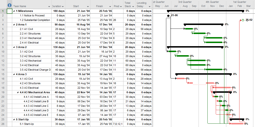
As shown below, these options lead to completely different schedules in the two tools, with MSP 2016 generating a leveled schedule that is 10-days shorter than the MSP 2010 version.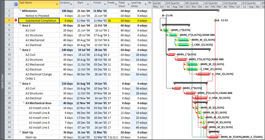

Key observations:

The MSP 2010 schedule failed to meet the Deadline, so more tasks are marked Critical due to zero-or-negative Total Slack. Six tasks including the two milestones have TS=-10d (i.e. the “most critical” as defined by Total Slack.)
The MSP 2010 leveler did not impose any task splits, even though they were allowed.
The MSP 2016 schedule meets the Deadline, so no negative slack is imposed. Seven tasks including the two milestones have TS=0 (the “most critical.”)
The MSP 2016 leveler imposed a task split on one task (A3 Structures).

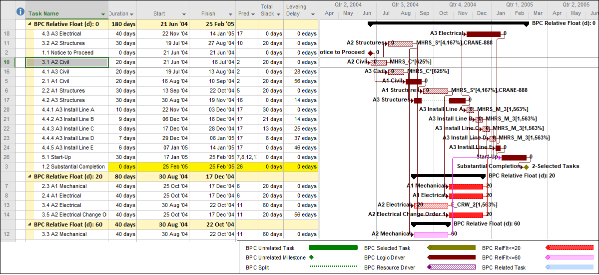
A close look at the Resource-leveled Critical and Near Critical paths – Using the Near Longest Path Filter in our BPC Logic Filter add-in – demonstrates that MSP 2016’s leveler creates a more condensed schedule. Specifically:

MSP 2010 generates a single continuous Resource-leveled Longest Path (BPC Relative Float = 0) comprised of eight tasks in sequence. The other 12 tasks possess 10 to 70 days of relative float.
MSP 2016 generates a continuous Resource-leveled Longest Path of 13 tasks in sequence, with 2 additional tasks (and a split part of one of the original 13) in parallel branches. The other 5 tasks possess from 20 to 60 days of relative float. As a result, more of the work is both concurrent AND Critical. It turns out that the splitting of the A3 Structures task is not the key to the more condensed schedule in MSP 2016. In fact, re-running the leveler while disallowing splits leads to a schedule that – with no splits and with a completely different sequential arrangement – finishes at the same time. The corresponding Resource-leveled Longest Path is comprised of only 8 tasks in sequence, with 1 additional, parallel/concurrent task. This leveled schedule has fewer resource mobilizations and disruptions along the longest path while still finishing at the earliest leveled time; it appears to be lowest risk.

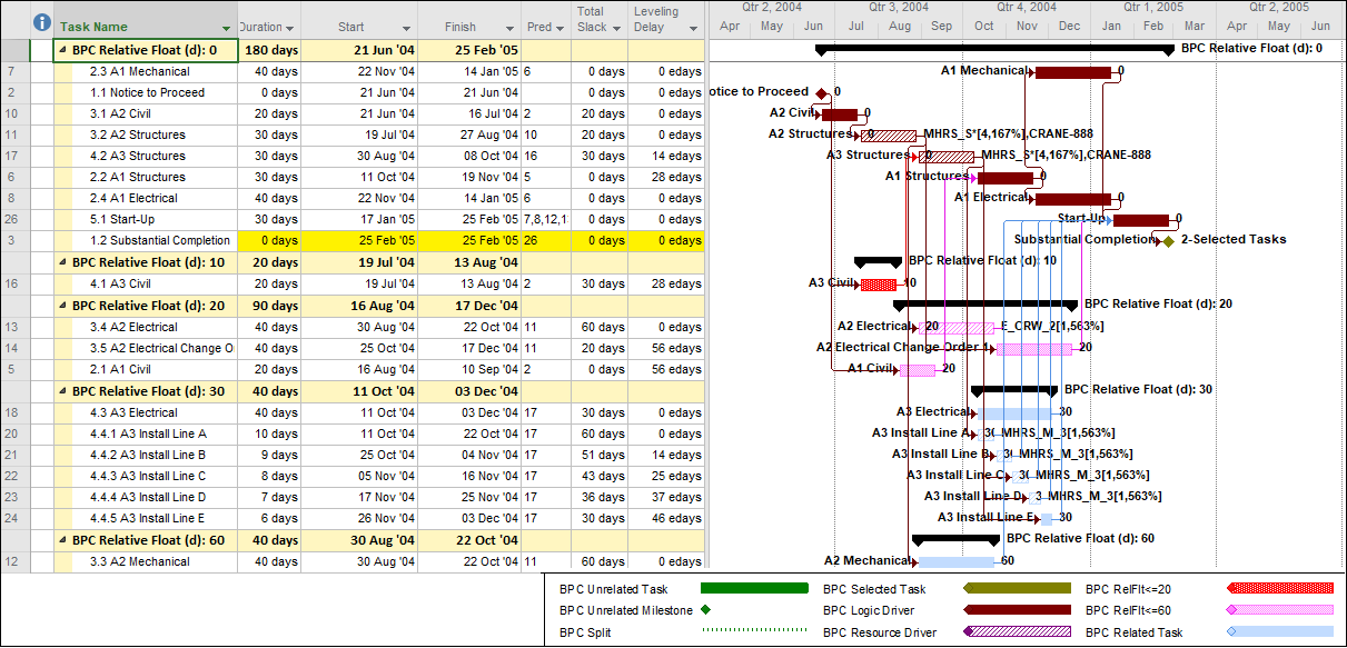
This example suggests that MSP 2016’s default resource leveling algorithm may be substantially more sophisticated than MSP 2010’s, and it promises – under the right circumstances – to offer shorter leveled schedules in the absence of explicit user-defined priorities. The shorter schedules may also be accompanied by technical and resource risks associated with multiple, concurrent branches of the resource-critical-path. Project managers using resource leveling are advised to consider and buffer these risks appropriately.

In contrast with this finding and in keeping with the prior version of this article, others have continued to observe consistently longer schedules being generated by MSP 2016 (compared to MSP 2010 and earlier), on some standardized schedule models. These observations are noted in the comments.

What is the Longest Path in a Project Schedule?

In Project schedules, the Longest Path yields the Shortest Time. Aside from the mental gymnastics needed to digest that phrase, the concept of Longest Path – especially as implemented in current software – has deviated enough from its origins that a different term may be needed.

Critical Path as Longest Path

Authoritative definitions of the “Critical Path” in project schedules typically employ the words “longest path,” “longest chain,” or “longest sequence” of activities … (that determine the earliest completion date of the project.) In other words, the path, chain, or sequence with the greatest measured length is the Critical Path. As a rule, however, none of the associated documents are able to clearly define what constitutes the length of a logic path, nor how such length will be measured and compared in a modern project schedule. Without a clear standard for measuring the length of something, explicitly defining the Critical Path in terms of the longest anything is just sloppy in my view.

The Original Path Length

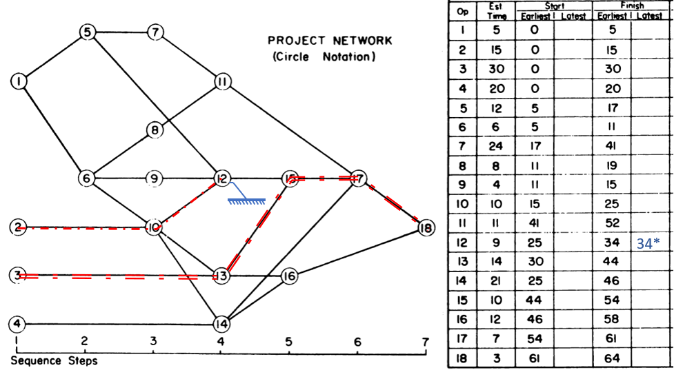
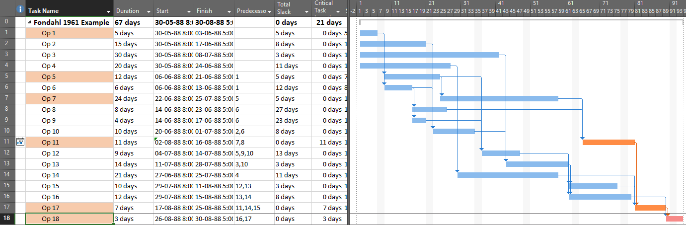
Assessing path length used to be much easier. In the early days of CPM (Critical Path Method) scheduling, any project schedule could be guaranteed to have ALL Finish-to-Start relationships, NO constraints, NO lags or leads, NO calendars, and only ONE Critical Path. Under these conditions, the length of a logic path could be clearly defined (and measured) as the sum of the durations of its member activities. Thus, the overall duration of a Project was equal to the “length” (i.e. duration) of its Critical Path, which itself was made up of the durations of its constituent activities. That result is indicated in the figure below, where the 64-day project length is determined by the durations of the 5 (highlighted) activities on the Critical Path. Adding up the activity durations along any other path in the schedule results in a corresponding path length that is less than 64-days – i.e. not the “longest” path. [The network diagram was taken from John W. Fondahl’s 1961 paper, “A Non-Computer Approach to the Critical Path Method for the Construction Industry,” which introduced what we now call the Precedence Diagramming Method. Unfortunately, Microsoft Project (MSP) has an early limit on dates, so his presumed ~1961 dates could not be matched.]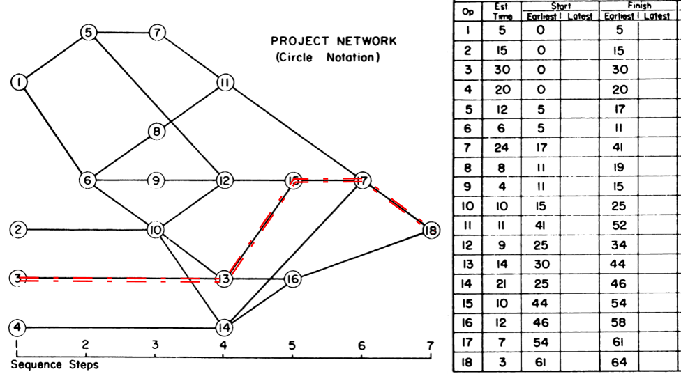

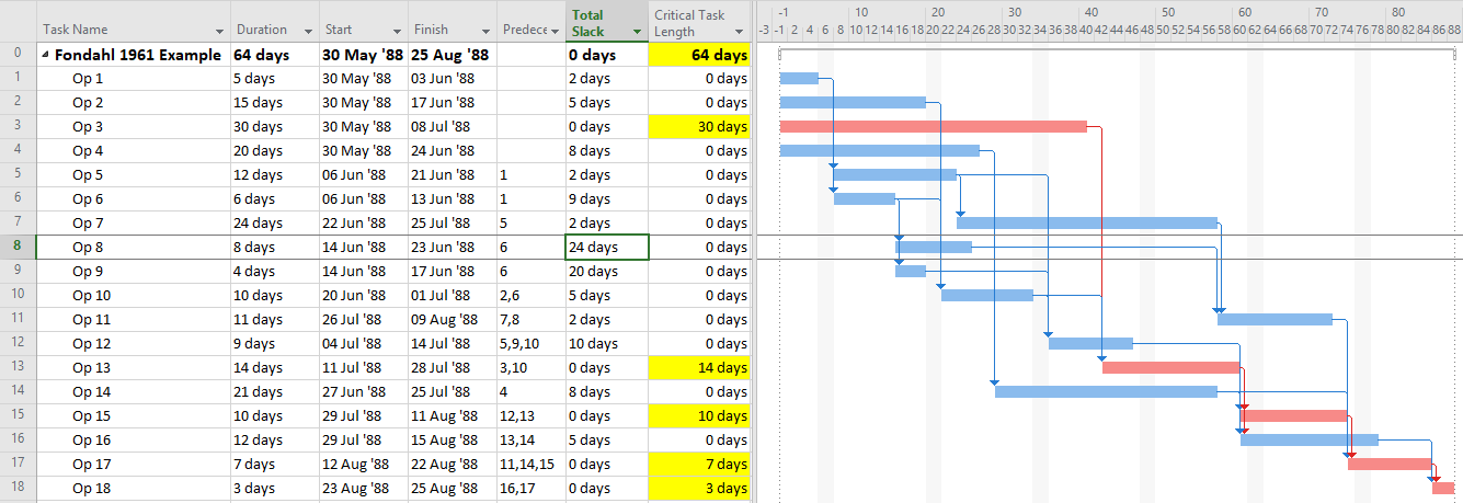
Fortunately, in such simple projects, it’s never been necessary to aggregate and compare the lengths of every logic path to select the “longest path.” The CPM backward pass calculations already identify that path by the activities with zero-Total Float/Slack, and successively “shorter” paths are identified by successively higher Total Float/Slack values. This fact has been verified in countless student exercises involving simple project schedule networks, typically concluding with the axiom that “the Critical Path equals the longest path, which equals the path of zero-Total Float/Slack.”

Float/Slack and Path-Length Difficulties

In general, modern complex project schedules have, or can be expected to have, complicating factors that make Total Float/Slack unreliable as an indicator of the Critical Path – e.g. non-Finish-to-Start relationships, various early and late constraints, multiple calendars, and even resource leveling. See this other article for details. Therefore, as noted earlier, the axiomatic definition has been shortened to “the Critical Path equals the longest path.”

Unfortunately, finding the “longest path” by arithmetically summing the activity lengths (i.e. durations) along all possible logic paths and comparing the results – not easy to begin with – has gotten more difficult. Lags, excess calendar non-working time, and resource leveling delays all add to the apparent “length” of a logic path compared to the simple summation of activity durations. Early date constraints may introduce delays that are not justified by task durations or logic relationships, breaking the path altogether. On the other hand, leads (negative lags), excess calendar working-time, and the use of overlapping-activity relationships (e.g. SS/FF) reduce its length. In addition, any hammocks, level-of-effort, and summary activities need to be excluded. All such factors must be accounted for if the “longest path” is to be established by the implied method of measuring and comparing path lengths in the project schedule. I don’t know of any mainstream project scheduling software that performs that kind of calculation. Alternatively, Deep Schedule Analysis^TM using the proprietary HCP (Hidden Critical Path) Method – from HCP Project Management Consulting – appears to compute and compare the lengths of all logic paths in Primavera and MSP schedules.

Longest Path as Driving Path

Contrary to summing up and comparing logic path lengths, most current notions of the “longest path” are based on an approach that does not involve path “length” at all. As a key attribute, the longest path in a simple, unconstrained and un-progressed project schedule also happens to be the driving logic path from the start of the first project activity to the finish of the last project activity. It is a “driving logic path” because each relationship in the path is “driving”, that is it prevents its successor from being scheduled any earlier than it is. Driving relationships are typically identified during the forward-pass CPM calculations. Subsequently, the driving path to the finish of the last activity can be identified by tracing driving logic backward from that activity, terminating the trace when no driving predecessors are found or the Data Date is reached. The resulting driving path to project finish is sometimes called the “longest path” even though its “length” has not been established. This is the “Longest Path” technique that has been applied for nearly two decades by (Oracle) Primavera and adopted more recently in other project scheduling tools.

As of today, MSP continues to define Critical tasks on the basis of Total Slack, but it provides no explicit method for identifying the “Critical Path” using a “longest path” criterion. How is the responsible MSP scheduler supposed to respond to a demand for the “critical path” when the longest path has been obscured? Here are several options:

Continue to make simple projects, avoiding all complicating factors like calendars (including resource calendars), early and late constraints, deadlines, and resource leveling. Then assume that “Total Slack = 0” correctly identifies the Critical Path.
If you are using MSP version 2013 or later,
- Ensure that your project is properly scheduled with logic open-ends only present at a single start and single finish task/milestone, then select the single finish task,
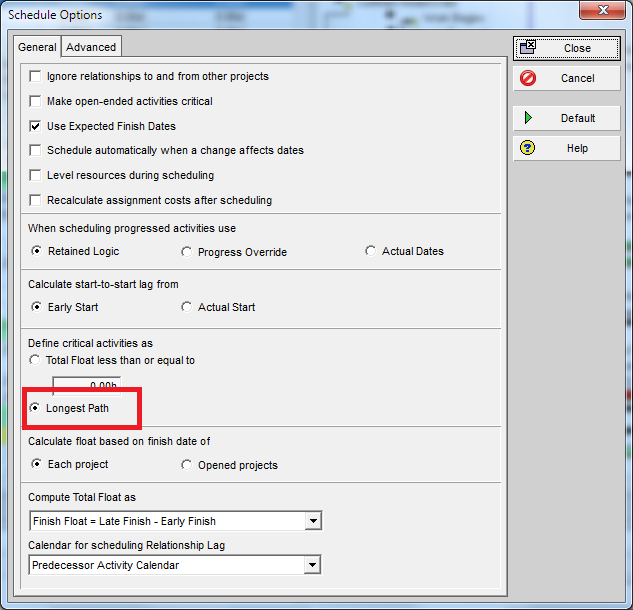
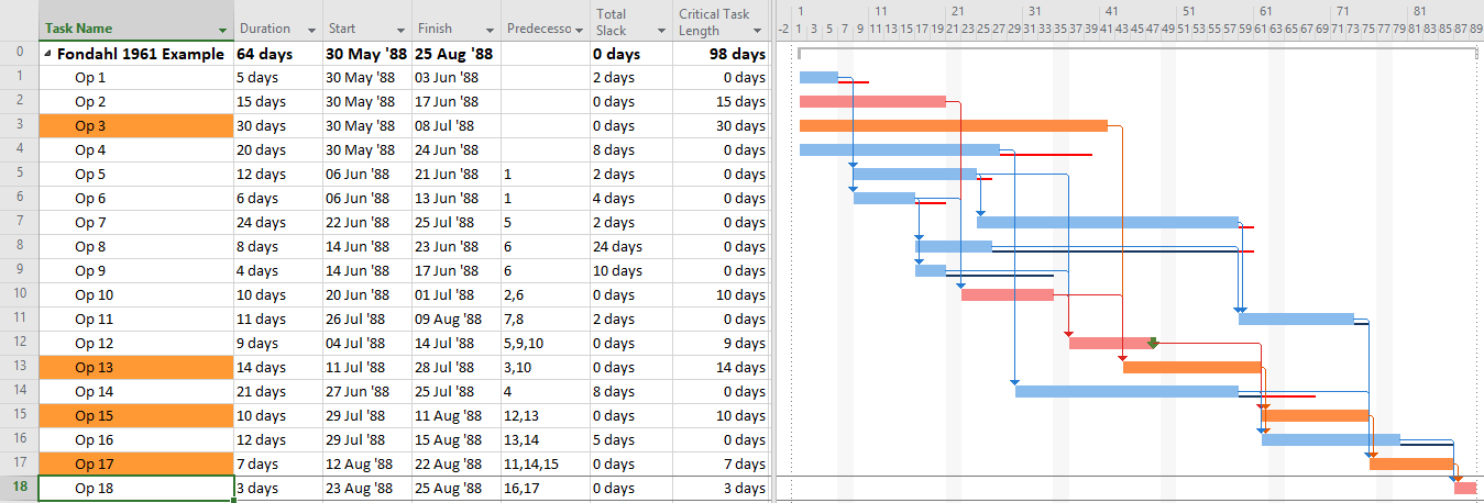
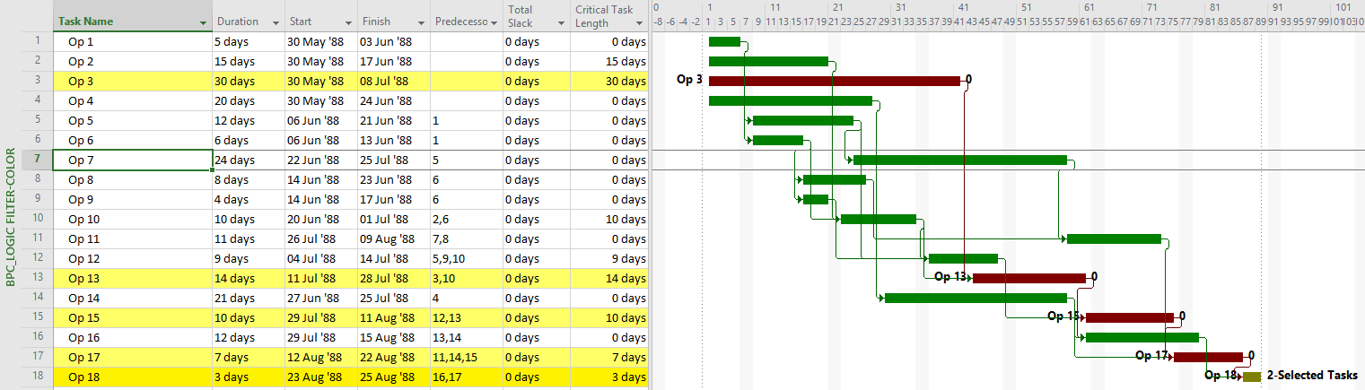
- Try to use the “Task Path” bar highlighter to highlight the “Driving Predecessors” of your selected finish task. In the example below, a Deadline (a non-mandatory late-finish constraint) has been applied to task Op12 in the 1961 example, and MSP has responded by applying the “Critical” flag (based on TS=0) to Op12 and its predecessors Op10 and Op2. As a result, the Critical Path is obscured. Applying the bar highlighter and selecting task Op18 (the project’s finish task) correctly identifies the driving path to project completion, i.e. the “longest path.” (For clarity, I manually added the corresponding cell highlighting in the table; the bar highlighter doesn’t do that.)
- If necessary, create and apply a corresponding filter for the highlighted bars. I’ve posted a set of macros to make and apply the filter automatically in this article.
If you are using MSP version 2007 or later,
- Ensure that your project is properly scheduled with logic open-ends only present at a single start and single finish task/milestone, then select the single finish task,
- Try to use the Task Inspector to identify the driving predecessor of the selected task, then go to it and flag it as being part of the driving path. Repeat this until the entire driving path is marked.
- If necessary, create and apply a filter and/or highlighting bar styles for the flagged tasks.
- I’ve posted another set of macros to do all this (except bar highlighting) automatically in this other article.
Note: The previous two approaches both rely on MSP’s StartDriver task object to identify driving relationships. As noted in this article, however, the resulting driving logic is not reliable in the presence of tasks with multiple predecessors, non-FS predecessors, or actual progress.
Use BPC Logic Filter or some other appropriate add-in to identify the “longest path” in the schedule.

Whichever method or software is used, expressing the Longest Path using the Driving Path methodology has one key weakness: it has not been proved generally useful for analysis of near-critical paths. While the Longest Path may be known, its actual length is not readily apparent. More importantly, there is no generally-accepted basis for computing the lengths, and hence the relative criticality, of the 2^nd, 3^rd, and 4^th etc. Longest Paths. Consequently, Near-Critical paths continue to be identified based on Total Float/Slack, which is still unreliable, or – in P6 – based on unit-less “Float Paths” from multiple float path analysis.

“Longest Path” and Early Constraints

As noted several times here, the methods described for identifying the “longest path” are in fact describing the “driving path to the project finish.” This distinction can raise confusion when one or more activities in the project schedule are delayed by an early constraint. Consider the case below, where an activity on the longest path (Op13) has been delayed 2 days by an early start constraint. Consequently, its sole predecessor relationship (from Op3) is no longer driving, and Op3 gains 2 days of Total Float/Slack. As shown by MSP’s “Driving Predecessor” bar highlighter, the driving logic trace is terminated (going backwards) after reaching the constrained task.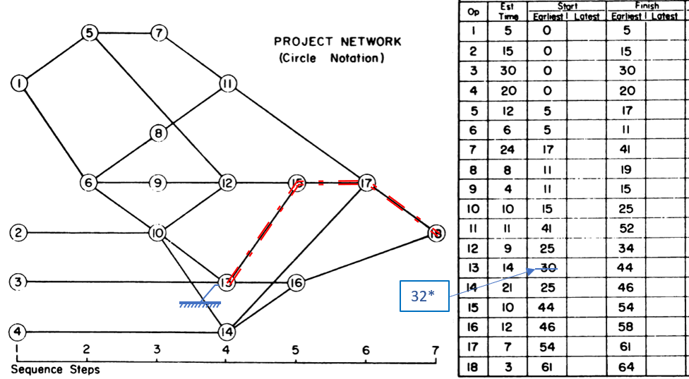

Identical results are obtained from Primavera’s (P6) Longest Path algorithm. This is neither surprising nor incorrect; the project’s completion is in fact driven by the external constraint on Op13, and its predecessor Op3 is quite properly excluded.

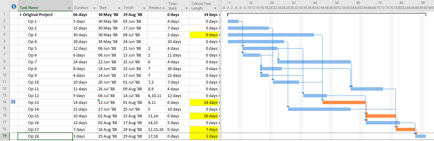
In this case, the application of an early constraint on a longest-path task simply truncates the longest path, which may be re-established using a logic tracing routine that jumps the constraint. In general, however, early date constraints can substantially change the driving path to project completion, such that the length (i.e. aggregate duration) of any particular logic path becomes irrelevant. For example, the next figure shows the consequences of imposing a one week (external) delay to Task Op11 in lieu of the earlier constraint. This leads to a 3-day delay of the project’s finish and a shift of the both the driving path and the zero-float path from Task Op13 to Op11. The total length of the corresponding critical path (including Op11’s formerly-driving predecessors) is 62 days. The 64-day path leading through Op13 and Op15 still exists, but it now has 3 days of total slack and is no longer driving the project completion. Thus, the mathematical longest path carries no significance in this constrained project schedule.

It’s clear therefore that the driving path to project completion and the longest path from the project start (or Data Date) to the project completion can differ when early constraints are present. P6’s “Longest Path” algorithm automatically defaults to the driving path, not the aggregate longest path, and to date there have been no built-in alternatives to that behavior. As a result, some consultants suggest that P6 Longest Path analyses should be rejected when external constraints – even legitimate ones like arrival dates for Customer Furnished Equipment – are present. Unfortunately, a position that requires strict duration-summing to identify critical (i.e. “longest”) paths in schedules containing early constraints appears to be both misleading and inconsistent with standard schedule calculating methods. (A P6 add-in, Schedule Analyzer Software, does claim to provide a true Longest Path representation in the presence of early constraints.)

BPC Logic Filter – Longest Path Filter

BPC Logic Filter is a schedule analysis add-in for MSP that my company developed for internal use. The Longest Path Filter module is a pre-configured version of the software’s Task Logic Tracer. The module is specifically configured to identify the project’s longest path (as driving path) through the following actions:

Automatically find the last task (or tasks) in the project schedule.
- Excluding tasks or milestones that have no logical predecessors. (E.g. completion milestones that are constrained to be scheduled at the end of the project but are not logically tied to the actual execution of the project. The resulting trace would be trivial.)
- Excluding tasks or milestones that are specifically flagged to be ignored, e.g. (“hammocks”)
Trace the driving logic backwards from the last task to the beginning of the project.
- Driving logic is robustly identified by direct computation and examination of relative floats. (Driving relationships have zero relative float according to the successor calendar.) The unreliable StartDriver task objects are ignored.
- Neither completed nor in-progress tasks are excluded from the trace.
Either apply a filter to show only the driving logic path, or color the bars to view the driving logic path together (in-line) with the non-driving tasks. The example below is identical to the previous one, but BPC Logic Filter formats the bar chart to ignore the impacts of the applied deadline. The resulting in-line view is substantially identical to the bar chart of the original, unconstrained project schedule.

BPC Logic Filter and the (True) Longest Path

As noted earlier, even a a single early constraint can truncate the driving path to project completion or change the driving path altogether. In either case, it is debatable in my view whether the addition of non-driving, float-possessing activities into the “longest path” makes that term itself more or less useful with respect to the typical uses of the “Critical Path” in managing and controlling project performance. If necessary, it is easy to add such activities – as unconstrained drivers of any constrained task – in BPC Logic Filter by checking a box. The bar chart below shows the results of the Longest Path Filter on the first early-constrained example schedule, as set up according to the driving-path (Primavera) standard. Results are identical to those of the built-in “Driving Predecessors” highlighter in MSP (above) and of P6.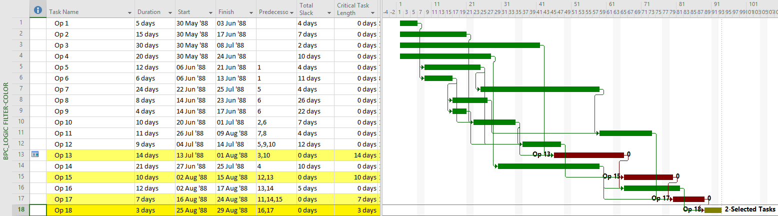

The next chart shows the complete “longest path” for the project, including the non-driving Op3 activity.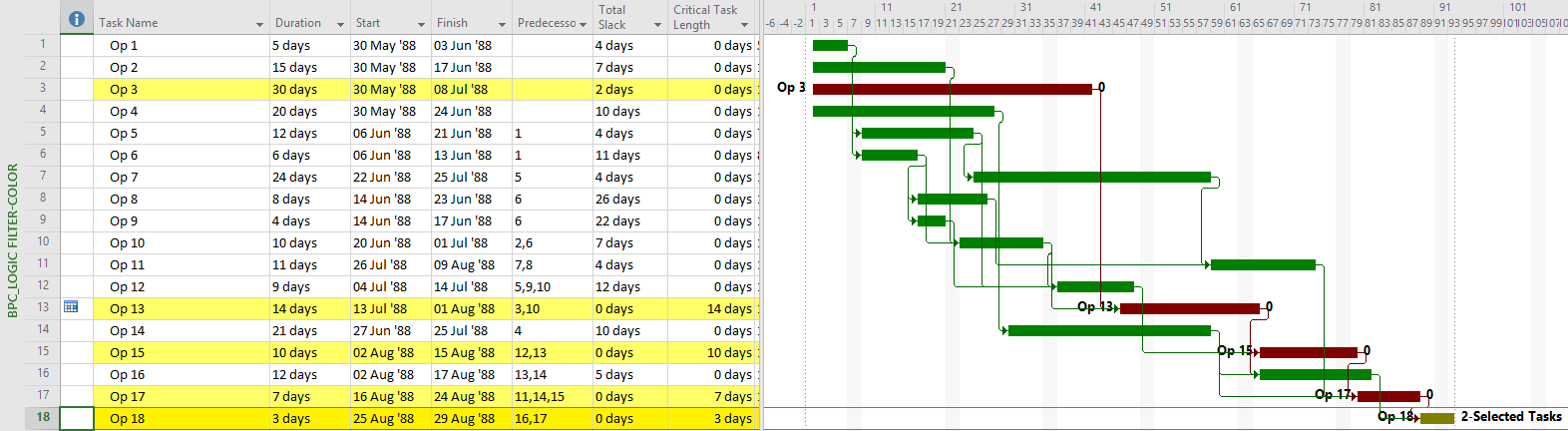

The second chart is different because the check box for “Override if successor task is delayed by constraint” has been checked in the analysis parameters form. Checking the box causes the non-driving predecessor with the least relative float to be treated as driving, and therefore included in the Longest Path, in the event of a constraint-caused delay.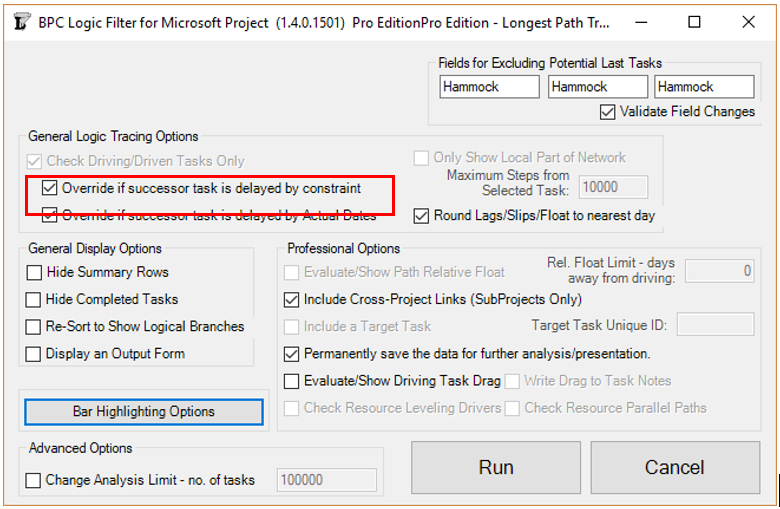

For a quick illustration, see Video – Find the Longest Path in Microsoft Project Using BPC Logic Filter.

BPC Logic Filter and Near Longest Paths

As noted earlier, the normal methods for identifying the “longest path” (i.e. the driving path) in a project schedule have not been generally adopted for analyzing near-longest paths. P6 offers multiple float path analysis, which I wrote about here. In addition, Schedule Analyzer (the P6 add-in mentioned earlier) computes what it calls the “Longest Path Value” for each activity in the schedule – this is the number of days an activity is away from being on the Longest Path (i.e. the driving path to project completion.) In the absence of demonstrated user demand, however, MSP seems unlikely to gain much beyond the Task Path bar highlighters.

BPC Logic Filter routinely computes and aggregates relative float to identify driving and near-driving logic paths in MSP project schedules. In this context, “near-driving” is quantified in terms of path relative float, i.e. days away from driving a particular end task (or days away from being driven by a particular start task.) Its “Longest Path” and “Near Longest Path” analyses are special cases where the automatically-selected end task is the last task in the project. For the Near Longest Path Filter, tasks can be shown in-line (with bar coloring) or grouped and sorted based on path relative float. The “override if successor is delayed by constraint” setting has no effect when the Near Longest Path Filter is generated. In that case, the non-driving task will be displayed according to its actual relative float. For example Op3 is shown below with a relative float of 2 days (its true value), not 0 days as shown on the earlier Longest Path Filter view.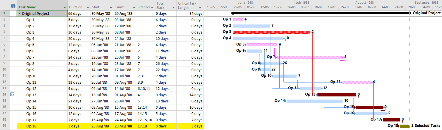

Recap

In the development of the Critical Path Method, the “longest path” originated as one of several defining characteristics of the “Critical Path” in simple project schedules. Specifically, the “Critical Path” included the sequence of activities with the highest aggregated duration – i.e. the “longest path”. Actual computation and comparison of path lengths was not necessary since relative path lengths could be inferred directly from Total Float – a much easier calculation.
Complicating factors in modern project schedule networks tend to confuse the interpretation of Total Float, such that it is no longer a reliable surrogate for path length. As a result, the most recent, authoritative definitions of the Critical Path tend to omit references to float while retaining references to “longest path” and, typically, logical control of the project completion date. [Notably, the measurement and comparison of aggregated path durations (path lengths) has not been an explicit feature of any mainstream project scheduling tool, so the “longest-path” part of the definition cannot be definitively tested in general practice.]
Notions of “longest-path” among current schedule practitioners are heavily influenced by the deceptively-named “Longest Path” feature in Oracle/Primavera’s P6 software. Perversely, that feature DOES NOT aggregate activity durations along any logic paths. Rather, it identifies the driving/controlling logic path to the project’s early finish date.
The “Longest Path” in P6 (i.e. the Driving Path to Project Completion) and the “longest path” (i.e. the logic path with highest aggregated duration) are NOT equivalent, particularly when the “Longest Path” is constrained by an early date constraint. There is at least one P6 add-in claiming to identify the true “longest path” (and near-“longest paths”) in this case.
Microsoft Project provides several inefficient methods to identify the Driving Path to Project Completion in simple projects, but these methods are not reliable in the presence of non- Finish-to-Start relationships. There are no native MSP methods for identifying near-driving tasks nor the true “longest path” in the presence of early date constraints. BPC Logic Filter is an MSP add-in that automatically fills these gaps.
As conceived, the “longest path” criterion implied the transparent calculation and comparison of aggregated activity durations along each logic path in a project schedule. As for Total Float, however, such calculations in complex schedules have been obfuscated by complications like non- Finish-to-Start relationships, lags, and multiple calendars. Since such obfuscation makes path lengths essentially un-testable, it appears that future Critical Path definitions should omit the “longest path” criterion in favor of a simple “driving path to project completion.”

Longest Paths in Backward Scheduled Projects (MSP) [Jan’19 Edit]

As pointed out in this recent article, the Longest Path in a backward scheduled project is essentially the “driven path from the project start,” not the “driving path to project completion.”

For more information, see the following links:

Article – Tracing Near Longest Paths with BPC Logic Filter

Video – Analyze the Near-Longest Paths in Microsoft Project using BPC Logic Filter

Avoid Out-of-Sequence Progress in Microsoft Project 2010-2016

[For the corresponding video presentation, see Construction CPM Conference 2020 – Avoid Out of Sequence Progress in Microsoft Project.]

Recording Actual dates that violate existing schedule logic can cause conflicts in Microsoft Project’s internal schedule calculations. The resulting Total Slack values and Critical task flags can be incorrect and misleading. These issues are aggravated by recent (e.g. MSP 2016) versions of the software, and users are advised to minimize out-of-sequence progress.

Recording of actual progress in a logic-driven project schedule can be problematic. As the “Actual” dates override or otherwise constrain the computed dates, the customary definitions of Float or Slack – and their resulting impacts on the “Critical” task flag in Microsoft Project (MSP) – no longer apply. While I hope to undertake a general review of progress updating issues in a future article, this one has a special focus on out-of-sequence progress for two primary reasons:

In all modern versions of Microsoft Project (e.g. ~MSP 2007+), the Total Slack values of “Critical” tasks with out-of-sequence successors can be altered unexpectedly.
In MSP 2016 (and possibly beginning with MSP 2013), the Total Slack values of ALL tasks (not just “Critical” tasks) with out-of-sequence progress among their successors can be altered unexpectedly. As a result, many tasks can be shown incorrectly as “Critical” in MSP 2016 when they are not “Critical” in earlier versions.

What is Out-of-Sequence Progress

Out-of-sequence progress exists when actual progress is recorded (via, e.g. Actual Start, Actual Duration, Actual Work, %Complete, etc.) at times when the logical constraints of the schedule would normally preclude it. For example:

An Actual Start is recorded for a task (the out-of-sequence, or OOS, task) whose Finish-to-Start predecessor has not finished. I.e. the Actual Start precedes the Early Start;
An Actual Start is recorded for an OOS task whose Start-to-Start predecessor has not started. Again, the Actual Start precedes the Early Start;
An Actual Finish is recorded for an OOS task whose Finish-to-Finish predecessor has not finished. Here the Actual Finish precedes the Early Finish.
An Actual Start is recorded for an OOS task whose Finish-to-Finish predecessor subsequently delays the completion of the work (on the OOS task). Again the Actual Start precedes the Early Start that would have existed in its absence.

In all cases there is a presumption that the recorded actual progress is more correct than the (theoretical) schedule model, so Early and Late dates are routinely overwritten by Actual dates during the schedule calculations. When the actual progress occurs out of sequence, however, computing the Late dates (and slack values) of incomplete predecessors (during the “Backward Pass” calculations) is complicated by logical conflicts. The software typically resolves these conflicts in a way that satisfies the needs of most users.

Completed, Out-of-Sequence Tasks

The issues discussed here are of primary concern in those cases where a task has started out of sequence and a) it remains incomplete; and b) the violated predecessor relationships remain unsatisfied (e.g. the FS predecessor remains incomplete.) If either the OOS task or its unfinished predecessor task become complete, then they are treated like other completed tasks in Microsoft Project. That is, they can influence the Early dates of their successors but have no impact on the Late dates of their predecessors. As a result of this latter condition, an incomplete task whose sole successor has been completed out of sequence becomes effectively open-ended, i.e. without successors. Under default conditions (i.e. “calculate multiple critical paths” NOT checked), the task’s Late Finish is set equal to the project’s Early Finish Date, and a high value of Total Slack is computed.

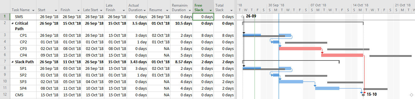
Obviously, this can have a major impact on the apparent Critical Path of a project. In the example below (which is further described in later paragraphs), tasks CP2 and SP2 have both been completed out-of-sequence, and at a duration of only 20% of their baseline durations. The overall project has been shortened, but the Critical Path has been truncated at CP3. CP1 is no longer “Critical” because, in effect, it no longer has any successors. It appears necessary to add a new FS relationship from CP1 to CP3 (and equivalently from SP1 to SP3) to re-establish the logic chain that has been broken by the completed, out-of-sequence tasks.

In Oracle Primavera P6, by contrast, the Retained Logic schedule setting automatically adjusts for activities completed out of sequence. Thus, the need to finish CP1 before proceeding with CP3 is already included. The result is a (presumably more realistic) 2-day delay in completion compared to the MSP result.

In-Progress, Out-of-Sequence Tasks

Key issues arise when the out-of-sequence task and its predecessor are both incomplete. Because this behavior is sometimes different for MSP 2016 than it is for MSP 2010, we’ll look at both versions for the remaining examples.

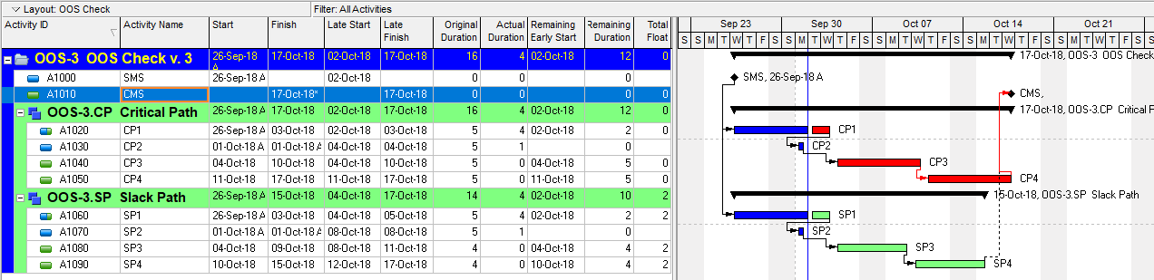
For exploring the behavior of in-progress, out-of-sequence tasks, we examine the simple project schedule below. The schedule is comprised of a single start milestone, a single finish milestone, a “Critical Path” string of four tasks, and a “Slack Path” string of four tasks. The “Slack Path” is two days shorter than the “Critical Path,” with the last two tasks each having a shorter duration. There is an unachievable Deadline applied to the finish milestone, and this creates negative Total Slack on the Critical Path. Thus, the Critical Path tasks all have TS=-1d, and the Slack Path tasks have TS=1d.

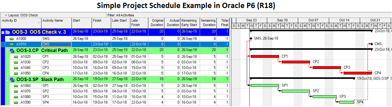
With no progress, the project is scheduled identically in both versions of MSP. Notably, P6 also starts with the same schedule dates.

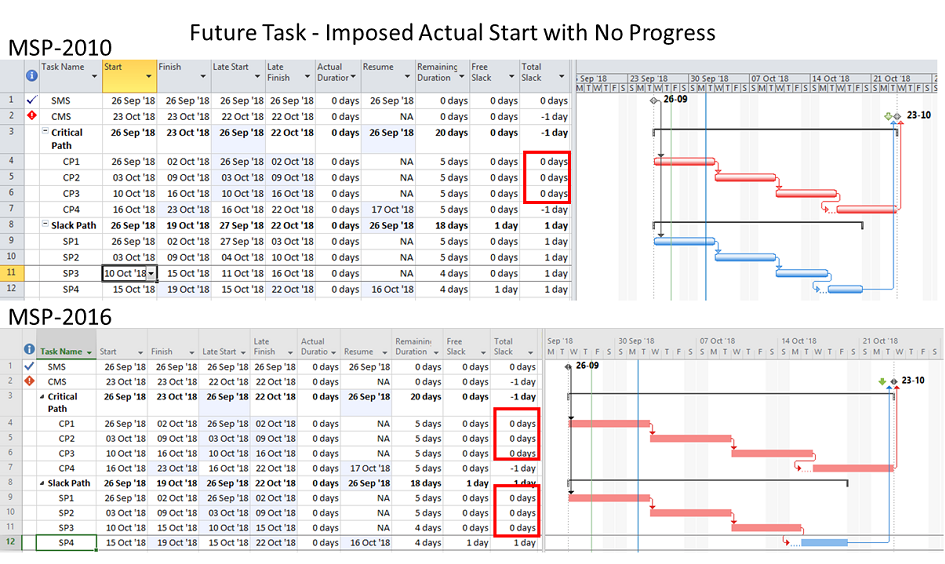
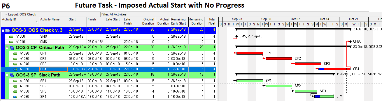
Now let’s examine what happens when we record an out-of-sequence Actual Start on some future task. In the example, the last task in each string (CP4 and SP4) is given an Actual Start that is one day earlier than its predecessors allow. To keep things simple, no progress beyond the actual starts are recorded (i.e. %Complete = 0%.) I’ve kept the “Split in-progress tasks” scheduling option checked (per default), so re-scheduling the project creates an initial split in tasks CP4 and SP4 and delays their remaining parts to satisfy the predecessor relationships. As a result, all the tasks keep the same finish dates as before, and the project finishes on the same date as before, one day after the Deadline.

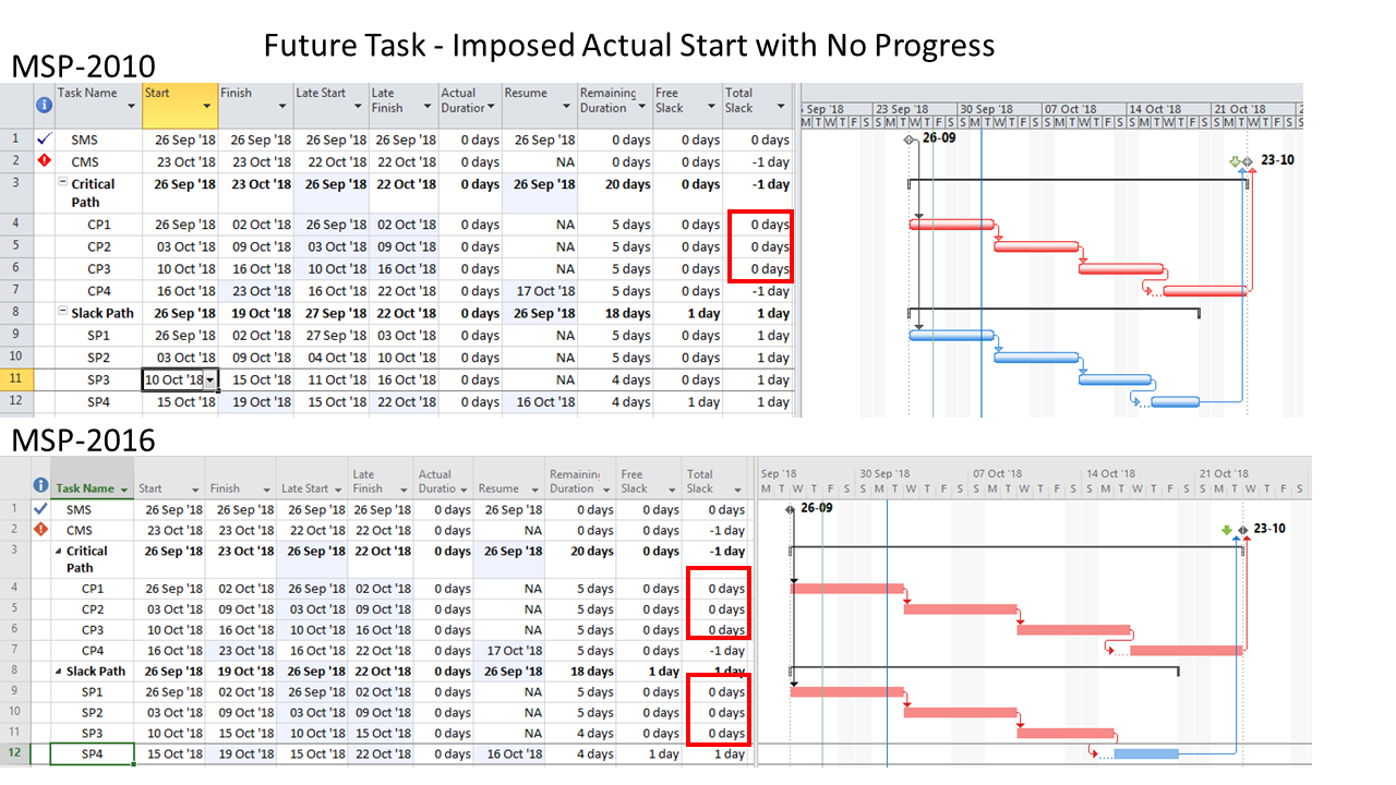
Although their start and finish dates have not changed, the logic-related information of the predecessors of the OOS tasks have been altered substantially.

In both MSP 2010 and MSP 2016:

The Total Slack values of the Critical Path tasks that precede the OOS task (i.e. tasks CP1, CP2, and CP3) are all changed from TS=-1d to TS=0d.
This behavior is not justified: if the tasks are all executed according to the scheduled dates, the project will still finish one day late. The tasks should still have TS=-1d.
This is in fact a general result (see also Comment 1): (Presumably for MSP 2007 through MSP 365), any super-critical (TS < 0) task with an out-of-sequence, in-progress task in its successor chain will automatically have its Total Slack re-set to zero. Thus, out-of-sequence progress can cause a task with 60 days of negative Total Slack to appear much less Critical than it is.
This behavior can present a problem for project managers operating in a negative-slack (i.e. behind-schedule) regime, where schedule-recovery efforts are typically prioritized based on Total Slack values. Entering a single OOS Actual Start value (whether correct or not), can substantially alter the overall schedule recovery picture.
It seems most MSP users pay no attention to Total Slack values beyond the application of the “Critical” flag, and the observed behavior doesn’t change that. Consequently, for most users up through MSP 2010, out-of-sequence progress appears to have no substantial impact on the “Critical Path.”

In MSP 2016, in addition to the prior behavior:
- In the example, the Total Slack values of the Slack Path tasks that precede the OOS task (i.e. tasks SP1, SP2, and SP3) are all changed from TS=1d to TS=0d.
- This behavior is also not justified. The tasks could all be delayed one day from their scheduled dates without compromising the project’s completion Deadline. The tasks should still have TS=1d.
- This is also a general result (see also Comment 1): (presumably for MSP 365 and maybe MSP 2013), ANY task (Critical or non-Critical) with an out-of-sequence, in-progress task in its successor chain will automatically have its Total Slack re-set to zero. Consequently, it will automatically and unavoidably be flagged as a Critical task.
- For general MSP users after MSP 2010, therefore, out-of-sequence progress can have a substantial, even major, impact. In particular, tasks that are actually far from the Critical Path may be incorrectly flagged as Critical.
The results in Oracle P6, however, appear more realistic. The Late dates and corresponding Float values are unchanged from the initial schedule.

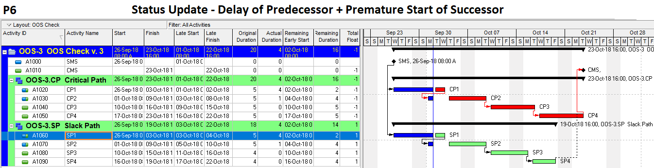
Below I’ve shown another perhaps more realistic example of the same simple project. There has been a simple progress update on the Status Date of 1Oct’18, four working days into the project. As of that date (the first Monday in the project), tasks CP1 and SP1 are still in-progress and have fallen one day behind the original plan. Their successors (CP2 and SP2) have been allowed to start early, however, with each recording one day of actual progress.

Similar logical results are observed. Task CP1 – the Critical predecessor of the Critical OOS task CP2 – now has TS=0d instead of TS=-1d in both software versions, and its Critical flag remains unchanged.

In MSP 2016 only, task SP1 – the non-critical predecessor of the non-critical OOS task SP2 – now also has TS=0d and is flagged as Critical. This is incorrect.

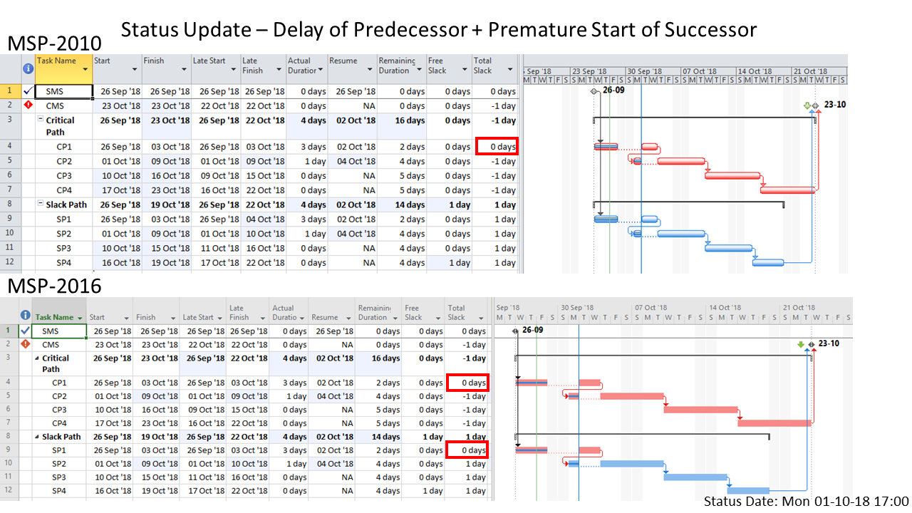
As before, however, the late dates and Float values in the P6 version of the schedule are aligned with expectations.

Out-of-Sequence Progress and Task Path Driving Predecessors in MSP 2016

The “Task Path” bar styles provide useful methods for identifying related tasks, including the Driving Predecessors path, for any selected task in MSP 2013+. The Driving Predecessors Task Path is particularly useful for confirming the Critical Path of a project when Total Slack is complicated by other factors. Unfortunately, the method is not successful when out-of-sequence progress is encountered. As shown in the figure below – repeating the two previous examples in MSP 2016 – the Driving Predecessors Task Path (orange-colored bars) is terminated when an Actual Start is reached on the backward (right-to-left) pass. Thus, driving Task Path functionality is not compatible with out-of-sequence progress.

[The Task Path functionality is equally incompatible with in-progress schedules that involve Finish-to-Finish relationships among overlapping tasks, even if none of the progress occurs out of sequence. Any Actual Start value terminates the progression of the associated bar formatting flag.]

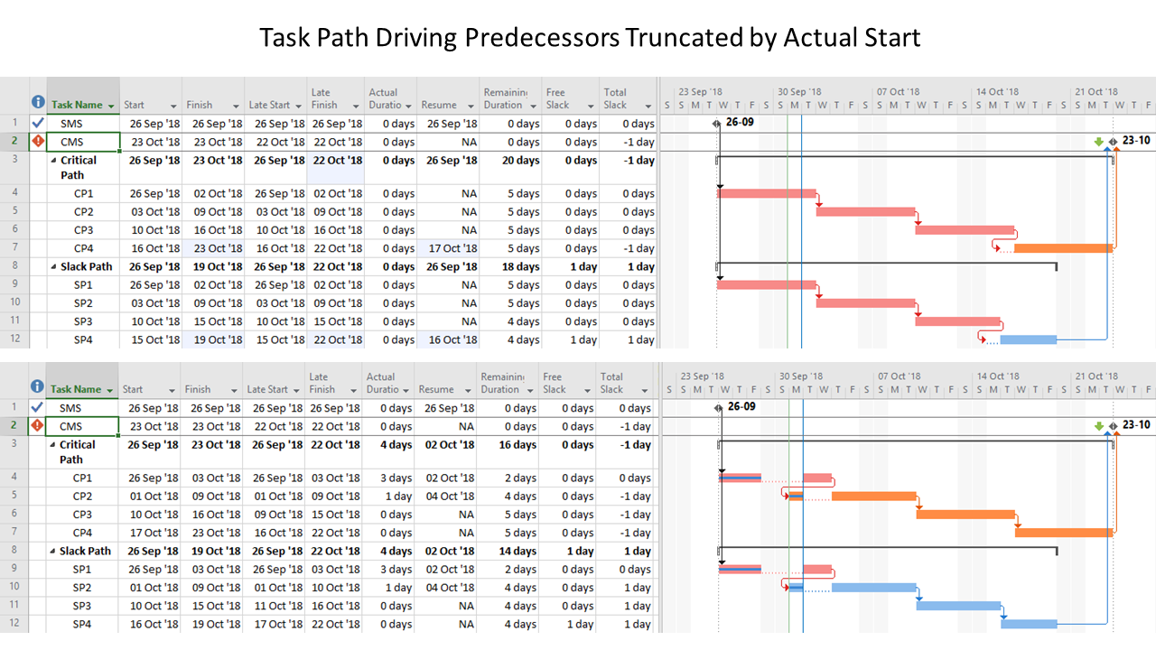
Out-of-Sequence Progress and BPC Logic Filter

The impacts of out-of-sequence progress on the Total Slack of some tasks are the result of specific decisions in MSP’s backward-pass algorithms for computing Late dates and Total Slack. Obviously, the algorithm has been tweaked between MSP 2010 and MSP 2016 leading to the even more undesired results.

BPC Logic Filter – my company’s MSP add-in for logic analysis – generally ignores MSP’s Deadlines, Late dates, Actual dates, and Total Slack values. Instead, it performs separate backward and forward traces to determine driving logic paths and relative float values. The latter, like Free Float, can never be negative. Thus, when BPC Logic Filter encounters out-of-sequence progress during a trace, zero relative float is applied, and a driving relationship is inferred. As shown in the examples below, this approach results in the correct identification of driving and near-driving paths to project completion, even when out-of-sequence progress is encountered. [In the bar charts, the path relative float is listed to the right of each bar. A zero-value represents the driving path with the bar characteristically colored (maroon), positive values and associated bar colors indicate the number of days away from driving the project completion.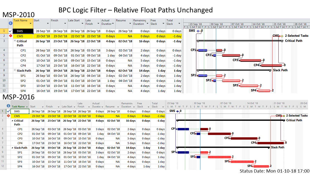

BPC Logic Filter also includes a Project Logic Checker to identify logic issues in Microsoft Project tasks. Like many such tools, it automatically flags OOS tasks, along with their immediate predecessors, for correction. (Beginning with release, 1.5.5.5, the tool also differentiates the important categories of OOS tasks. The “-I” suffix in the bar chart below identifies out-of-sequence conditions where both predecessor and successor of the violated relationship remain Incomplete; total slack in such cases cannot be trusted.)

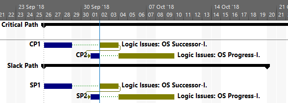
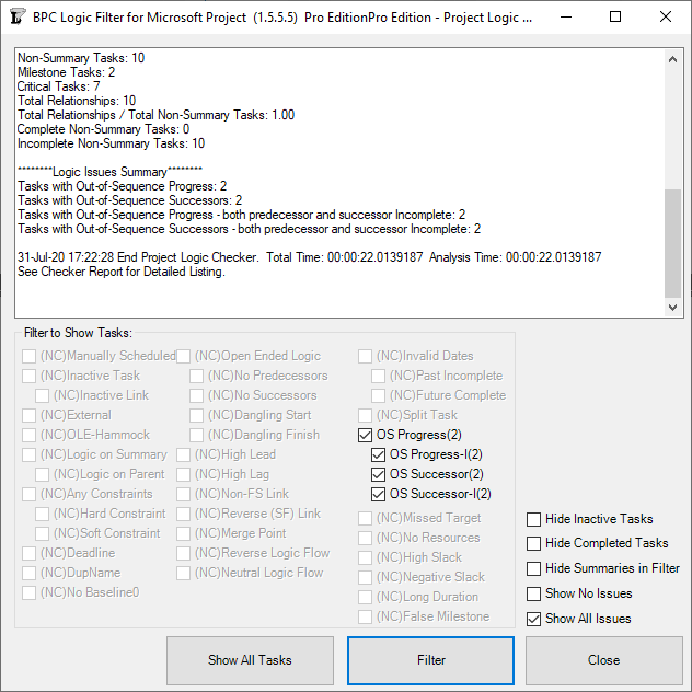
In addition, the Logic Inspector in BPC Logic Filter automatically flags tasks with out-of-sequence progress as well as all the relationships that are violated by such progress. Here it is shown that the out-of-sequence progress on task SP2 violates its predecessor relationship with SP1. The late dates and total slack of the predecessor (SP1) are incorrect.

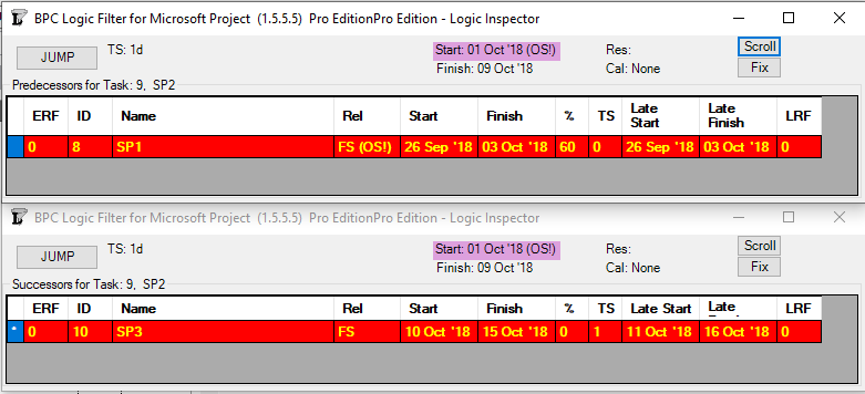
Out-of-Sequence Progress in the Real World

This examination was prompted by an associate who, after a recent “upgrade” from MSP 2007 to MSP 2016, encountered numerous unexplained changes in the “Critical Path” during project updating. As it turned out, the updated schedule contained extensive out-of-sequence progress that explained the observed behavior. The out-of-sequence progress was the result of a schedule model that was ultimately invalid – a poor representation of the work, either as planned or as actually executed. As is often the case in construction, this was aggravated by the persistent executive schedule pressure that converts some technological restraints (e.g. don’t start interior finishes until the building roof and skin are closed up) from mandatory requirements into mere preferences.

A typical invalid schedule model involves the representation of multiple overlapping activities as an over-simplified Finish-to-Start string. For example, the schedule below shows five sequentially-related, non-critical tasks, of roughly equivalent work content, that are scheduled to occur over a five-week period. Although they are shown sequentially, it is in fact customary to execute these five tasks nearly concurrently, with each task commencing as soon as its predecessor’s progress allows – and thereafter suspending or pacing progress to match that of its predecessors.

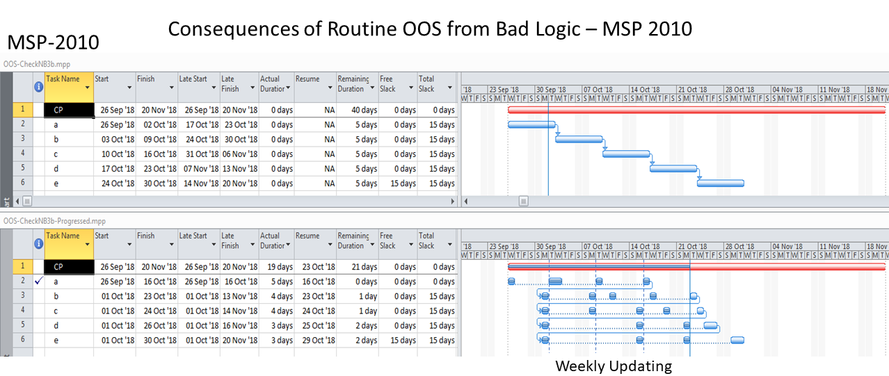
[Some schedule purists would suggest that these tasks should be broken down into many small, repetitive work packages, all arranged with pure Finish-to-Start logic relationships. The resulting schedule is extremely detailed and reflects a true logical plan for executing the work. In my experience, however, such a detailed plan can often be riddled with preferential logic that is ultimately over-ruled by field decisions. Out-of-sequence progress – in spades – is the inevitable result; the scheduling workload multiplies with no added value.

Another approach might involve five parallel tasks, each of five weeks duration, modeled with continuous relationships or at the very least with compound (joint SS + FF) relationships. Unfortunately, neither relationship is supported by MSP. The dummy-milestone approach that I use to mimic compound relationships in MSP seems fairly esoteric, and the common alternative – using solely SS or FF relationships – can be problematic.]

The scheduler here has chosen the most expedient route, a simplified Finish-to-Start string of five activities. Four weekly updates of actual progress then lead to the progressed schedule shown at the bottom of the figure. While its appearance is substantially changed compared to the original plan, the progressed schedule – in MSP 2010 – seems to correctly depict the status and slack of the multiple in-progress, out-of-sequence tasks. Thus MSP 2010 seems largely indifferent to the consequences of invalid logic combined with out-of-sequence progress, as long as the affected tasks are non-critical.

As my associate discovered, however, MSP 2016 is far less tolerant of such practices. When the progressed schedule is recalculated in MSP 2016, the in-progress predecessors of the in-progress, out-of-sequence tasks are shown as Critical (with TS=0). This is incorrect, as the tasks could all slip by 15 days without delaying the project.

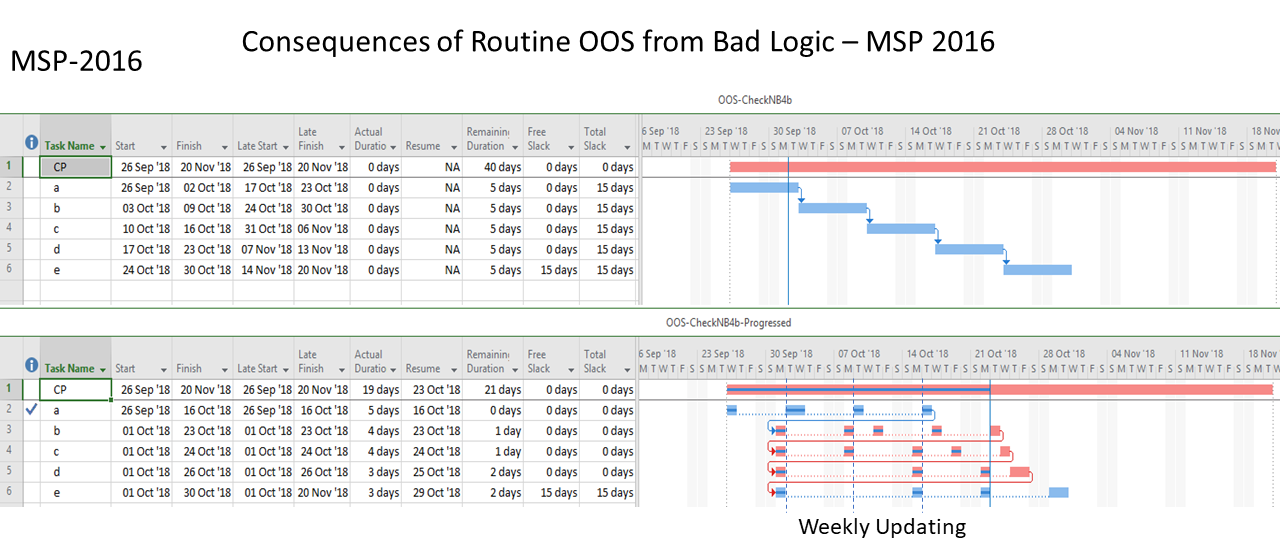
For comparison, here are the corresponding updates for the identical project schedule in Oracle P6 (R18.8.10). The dates and Float values are identical to those for MSP 2010; they are correct for these non-critical tasks. (Original and Actual Durations in P6 are handled differently than in MSP, so those are not comparable.)

Review and Recommendations

Out-of-sequence progress is an unwelcome but often unavoidable occurrence in projects with logic-driven schedules. It happens when the actual project execution is allowed to deviate from the plan in a way that creates logical conflict in the automatic scheduling calculations. It typically results from a combination of the following circumstances:

The schedule plan includes logic relationships that are not technologically mandatory. I.e. there are a number of alternative methods available for sequencing a group of related activities, and only one (preferred) method is incorporated into the schedule. In addition:
- Procedural controls are inadequate to ensure that project execution conforms to the preferred logic sequence; or
- Subsequent to initial schedule development, the preferred logic sequence is altered due to field conditions, resource limitations, or other factors.
Subsequent to initial schedule development, technologically-mandatory logical constraints are allowed to be violated – typically under schedule performance pressure – and the resulting technical risks are accepted.
The schedule is based on scope and logic definitions that are overly simplified compared to the actual or achievable plan of execution. E.g. simple Finish-to-Start relationships are used to represent overlapping, partly-concurrent activities.
Subsequent to occurrence of any of the prior circumstances, the schedule logic is not revised appropriately.
Schedule updates do not include regular review and correction of invalid logic in light of out-of-sequence progress.

In MSP, a task that is both started and completed out-of-sequence may cause the incomplete tasks in its predecessor and/or successor chains to become effectively open-ended, with impacts on Early and Late dates, Total Slack, and Critical task definition. Consequently, the updated schedule may be invalid.

A task that is started out-of-sequence but remains in progress may cause substantial alterations to the Late dates, Total Slack, and Critical definitions of the incomplete tasks in its predecessor chains. In particular:

(In all modern MSP versions) Total Slack of behind-schedule tasks will change from negative to zero and in some cases turn positive. [See also comment 1.] Although the Critical flag won’t always change, any identification of driving and driven logic paths that is based on negative Total Slack will be incorrect.
(In recent versions – e.g. MSP 2016) Total Slack of non-Critical tasks will change from positive to zero (with some exceptions), and each task will be incorrectly marked as Critical. [See also comment 1.] Thus, the “Critical Path” and any other Slack-based identification of driving or driven logic paths will be incorrect.

These are pretty major consequences, yet their persistence suggests that they reflect as-designed behavior, not bugs. It might even be suggested that the most recent “improvements” are intended to highlight the out-of-sequence progress – for correction of the associated logic.

In MSP, the only reliable way to avoid the negative consequences of out-of-sequence progress, in my opinion, is to avoid and/or minimize its occurrence. Fundamentally, this means:

Ensure that project schedules are based on sound consideration of the scope and logic of project execution.
Ensure that procedural controls are put into place to a) validate, b) revise where necessary, and c) enforce the preferred sequence of activities.
Where necessary, revise the schedule logic to reflect the actual/required sequence of execution.
During regular progress updates, identify all out of sequence progress, and revise associated logic as appropriate to avoid the consequences noted above.