Alternate Definitions of Driving Logic Relationships in Project Schedules

[Article 2 of 2.] This is a summary of the alternate definitions and uses of driving logic relationships between activities in project schedules, as applied in Primavera P6 and Microsoft Project software.  Driving relationships are often considered fundamental elements of the project critical path.

This winter I worked with a colleague to prepare a paper – Interpreting Logic Paths in Multi-Calendar Project Schedules – for presentation at this year’s AACE International Conference and Expo in Chicago (Covid-19) virtual world.  It’s a deep dive into the Multiple Float Path calculation options in Primavera P6 scheduling software.  During the technical study, I had a lot of opportunities to think about driving logic relationships.  I’ve summarized the standard definitions and uses in an earlier article.  This entry summarizes the alternate versions of driving logic relationships that sometimes arise.

The Importance of Driving Logic

The planning and execution of complex projects requires the project team to understand, implement, and communicate the consequences of schedule logic flow to the other stakeholders.  Through schedule logic, each activity in the project has the potential to constrain or disrupt numerous other activities – and to be constrained or disrupted by them.  The most obvious artifacts of logic flow are the important logic paths, like the critical path, the Longest Path (in Primavera P6), or the driving path to a key delivery milestone.  Regardless of the detailed definition, each of these important paths is governed by driving logic relationships from the first activity to the last activity in the path.

Late-Dates and Bi-Directional Driving Relationships in Primavera P6

From the earlier article, a relationship is considered driving (under the standard definitions) when its successor’s early dates are constrained by the relationship, during the forward pass of the CPM calculations.  That is, standard driving relationships are early-dates driving relationships.  A late-dates driving relationship, in contrast, is one that constrains the late dates of the predecessor, during the backward pass.  When an activity has multiple successors, then one or more of these successor relationships may be controlling the late dates, and hence the total float, of the selected activity; this is a late-dates driving relationship.

Identification of late-dates driving relationships is a key factor in P6’s Multiple Float Path (MFP) calculation.  Under the total float calculation option, a relationship can be assigned to a driving “float path” only if it meets the criteria for both early-dates and late-dates driving relationships.  That is, it possesses bi-directional driving logic.  Since P6 does not flag or otherwise mark such relationships, the results of multiple float path calculations with the total float option can be confusing.  Full understanding of the float paths may require a detailed examination of relationship and activity floats, especially when multiple calendars or constraints are involved.

For more information on MFP calculations in P6, check out these other entries in the blog:

Beyond the Critical Path – the Need for Logic Analysis of Project Schedules

P6 Multiple Float Path Analysis – Why Use Free Float Option

Relationship Free Float and Float Paths in Multi-Calendar Projects (P6 MFP Free Float Option)

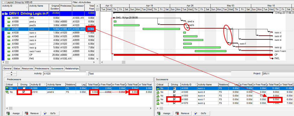
Aside from the MFP calculation option in P6, this type of driving logic is useful mainly for prioritizing driving successors when click-tracing through the schedule network in the forward direction – perhaps for schedule validation or disruption analysis.  For example, consider the selected activity (A1020, “Task”) in the P6 version of our simple project below.  A glance at the late-date bars shows that only one of its five driven successors (A1060, “succ f”) is responsible for the late dates (and total float) of the selected task.  The corresponding relationship possesses bi-directional driving logic and marks the forward continuation of the total-float-based driving path.  In the relationship tables, the “Driving” checkboxes already indicate the relationships with early-dates driving logic.  When exploring forward, most P6 users will simply click to the driven successor activity that is “Critical” or has the lowest total float value, and that will be correct much of the time.  When multiple constraints and/or calendars exist, however – or when the path being explored is far from critical – then late-dates driving logic is indicated when the “Relationship Total Float” equals the total float of the predecessor activity, as highlighted in the figure.

Late-Dates and Bi-Directional Driving Relationships in BPC Logic Filter

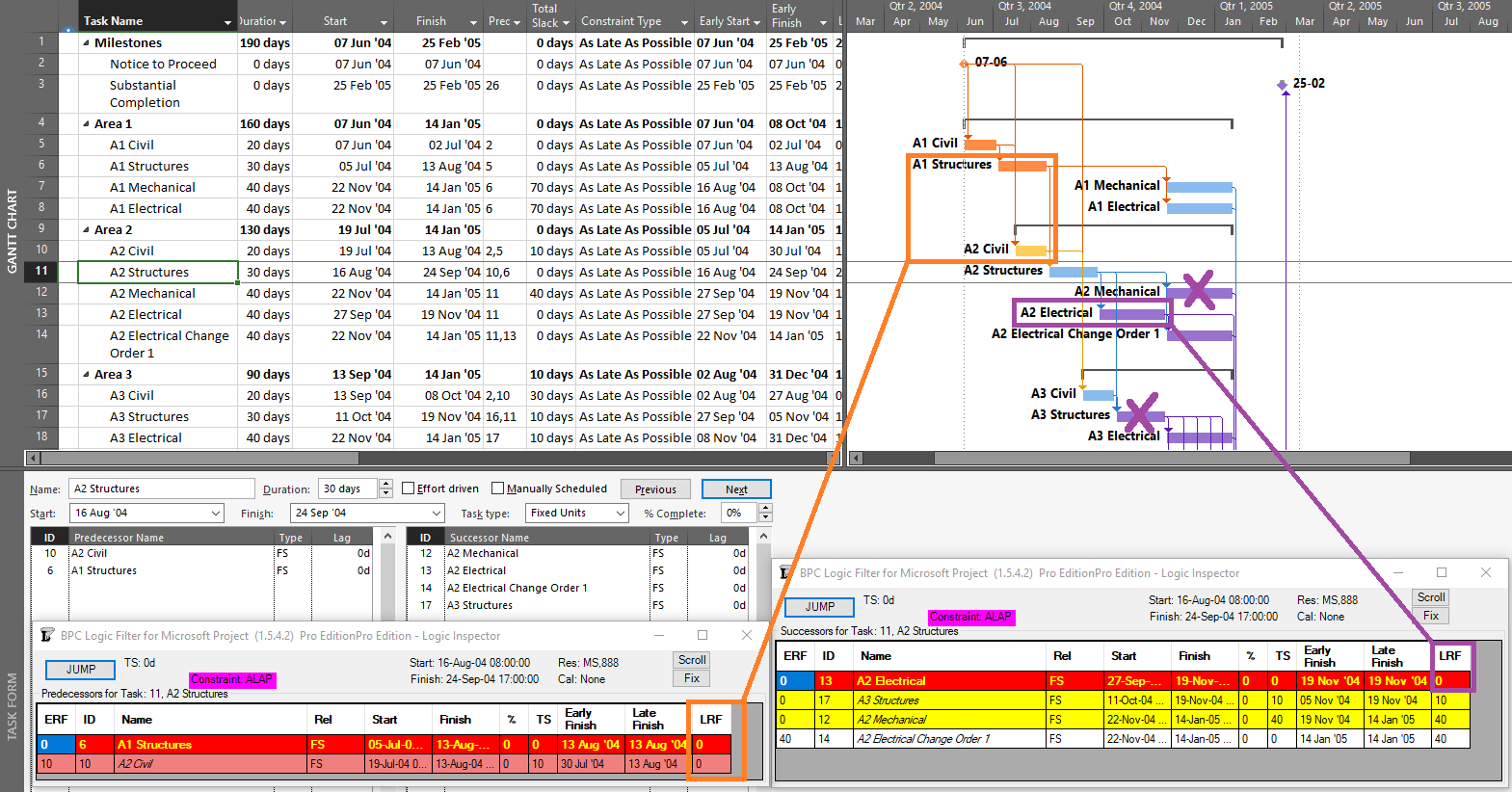
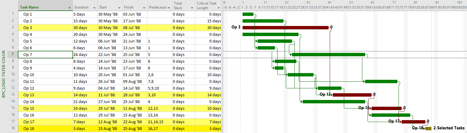
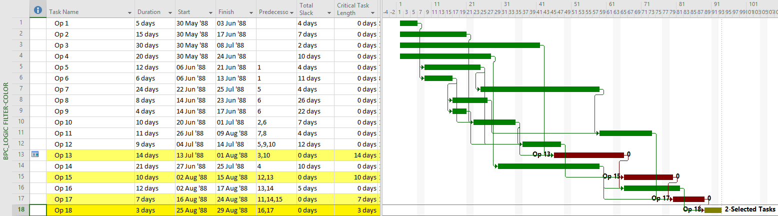
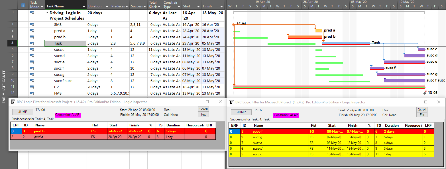
With no built-in alternatives, BPC Logic Filter automatically identify all three types of driving relationships – early-dates, late-dates, and bi-directional – in Microsoft Project schedules.  The next figure repeats the same simple example project from the earlier article, with additional bars for early and late dates (green and red) and the task paths shown earlier (orange, gold, purple.)  Within the logic inspector tables, bi-directional driving relationships are highlighted (red/yellow) and shown on top.  Among those relationships that are NOT bi-directional drivers, early-date drivers are shown in the same yellow as before, and late-date drivers are shown in pale red.  As usual, the logic inspector’s jump buttons make for easy, logic-based navigation through the schedule.

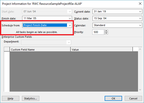
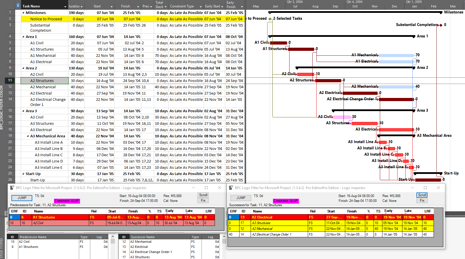
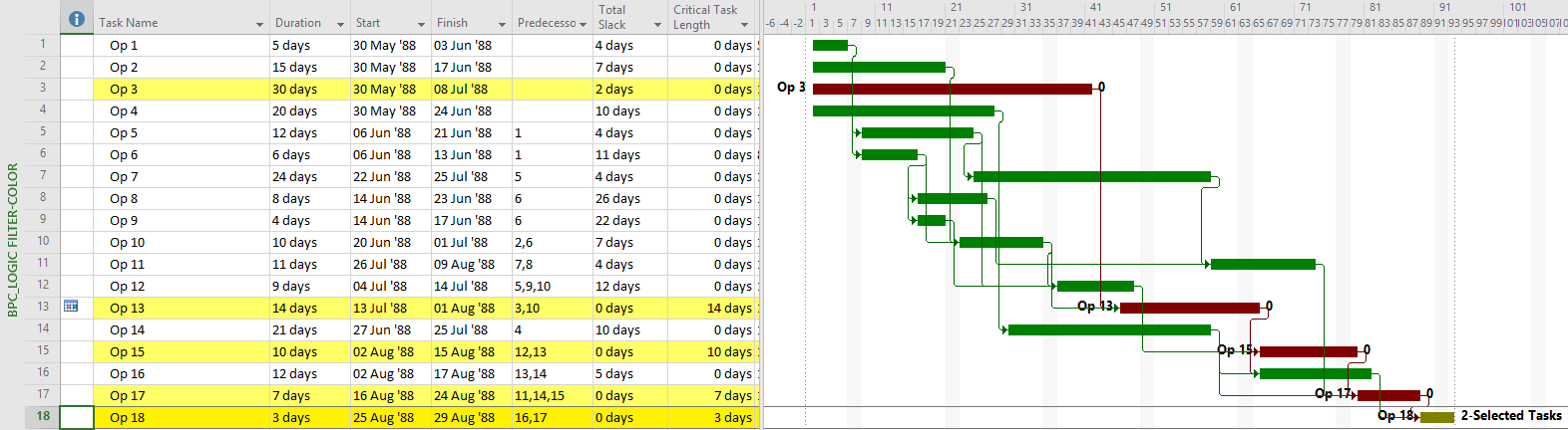
Unlike MSP’s built-in task path bar styles, the logic inspector tables are equally effective at illustrating driving logic in backward-scheduled projects.  This is demonstrated below, where the same example project has been re-configured to Schedule from: Project Finish Date.  Interestingly, while the scheduled dates clearly change, the nature of driving logic relationships does not.

For further information on driving logic in backward-scheduled projects, check out this earlier entry:  Driving Logic in Backward Scheduled Projects (Microsoft Project), which pre-dated the introduction of late-dates driving calculations in the logic inspector.

Resource Driving Logic Relationships in BPC Logic Filter

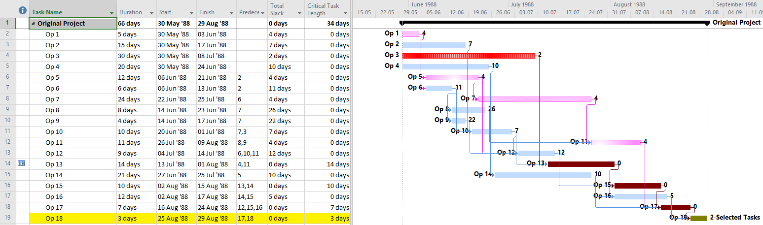
When resource leveling is imposed in a P6 or MSP project schedule, some tasks are delayed from their CPM-based early dates until resources become available – after completion of other tasks.  In the figure below, a single resource has been assigned to the five successors of the “Task,” and the resulting overallocation of the resource has been resolved by leveling the schedule using the simplest options.  As a result, the project finish milestone has been delayed by three days, and the critical path has shifted.

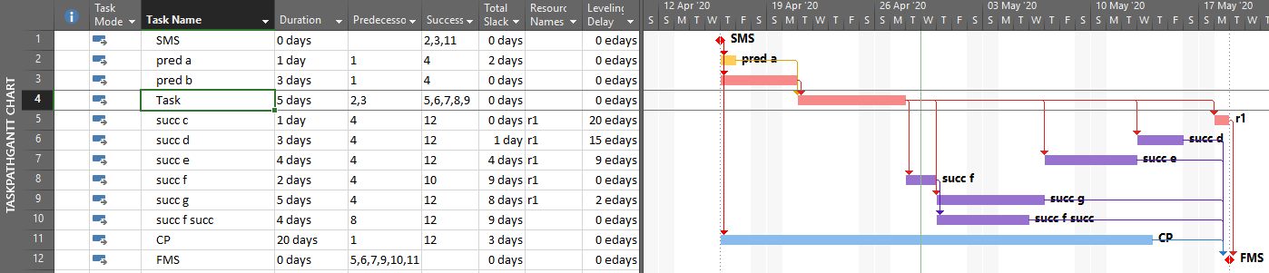
The leveling process creates implied driving relationships between tasks that demand the same resources.  BPC Logic Filter infers these “ResDrvr” relationships.  As shown below, the resulting resource-constrained driving logic paths are typically very different from those identified using CPM logic alone.

The consequences of resource driving logic are further addressed in these earlier articles:

Resource Leveling Breaks the “Critical Path” – Logic Analysis of Resource-Leveled Schedules (MS Project)

The Resource Critical Path – Logic Analysis of Resource-Leveled Schedules (MS Project), Part 2

Hierarchical (Parent-Child) Driving Logic Relationships in Microsoft Project

Unlike other project scheduling tools, MSP supports direct assignment of schedule logic (start predecessors and finish successors only) to “summary tasks.”  As a consequence, it then imposes automatic logic restraints based on the relative positions of tasks within the Outline/Work breakdown structure.  Thus, a summary task with a finish-to-start predecessor automatically imposes a corresponding early-start restraint on every one of its subtasks, and this restraint is inherited at each outline level all the way to the lowest-level subtask.  Moreover, a summary task with a finish to start successor automatically imposes a corresponding late-finish (backward-pass) restraint on its subtasks, which is inherited all the way down the outline structure.  External date constraints, manual-mode scheduled dates, and actual dates inputs for summary tasks have similar consequences.

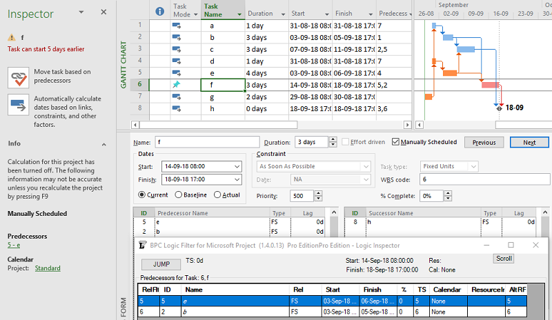
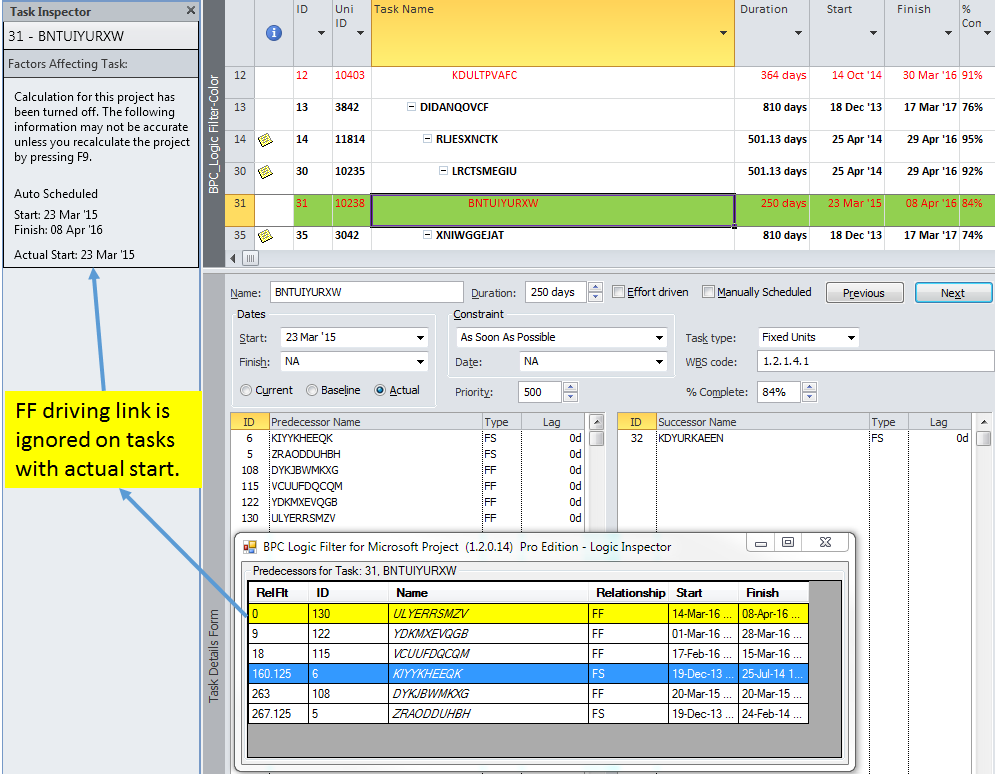
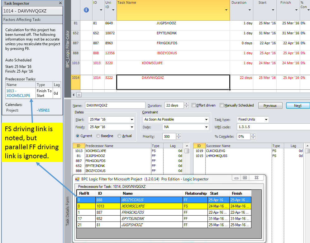
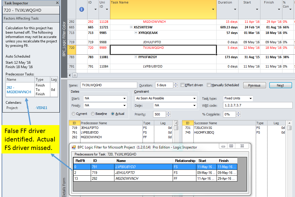
The immediate early-start drivers for summary tasks and subtasks – whether a result of predecessor logic, outline-parent inheritance, or outline-child roll-up – can be identified by the task Inspector as shown in the next figure, and some of these are explicitly enumerated in the “driver” collections of the task.  The late-date consequences remain implicit, however.

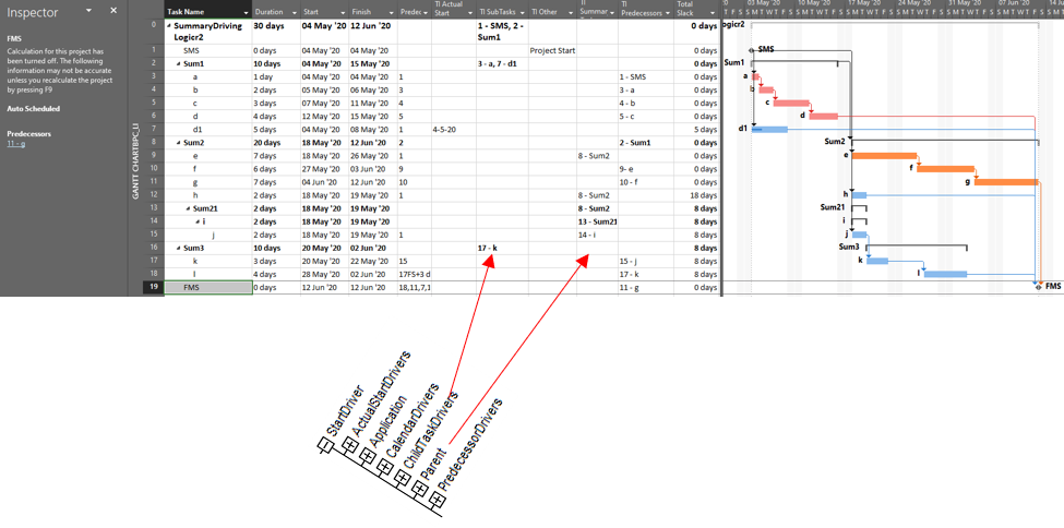
The apparent critical path for the schedule of the previous figure runs through tasks a-d and tasks e-g, including their driving FS relationships.  Not shown, however, is the implicit driving FF relationship from task d to its outline parent task Sum1 (here identified in BPC’s logic inspector tool.)

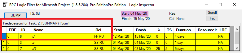
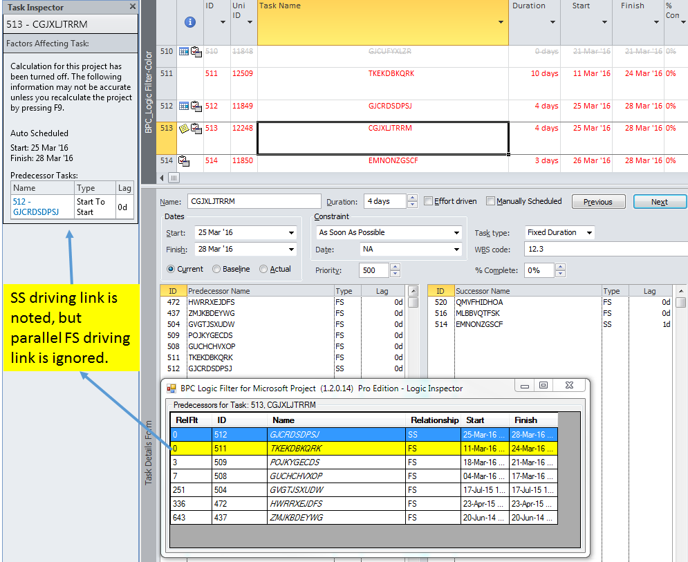
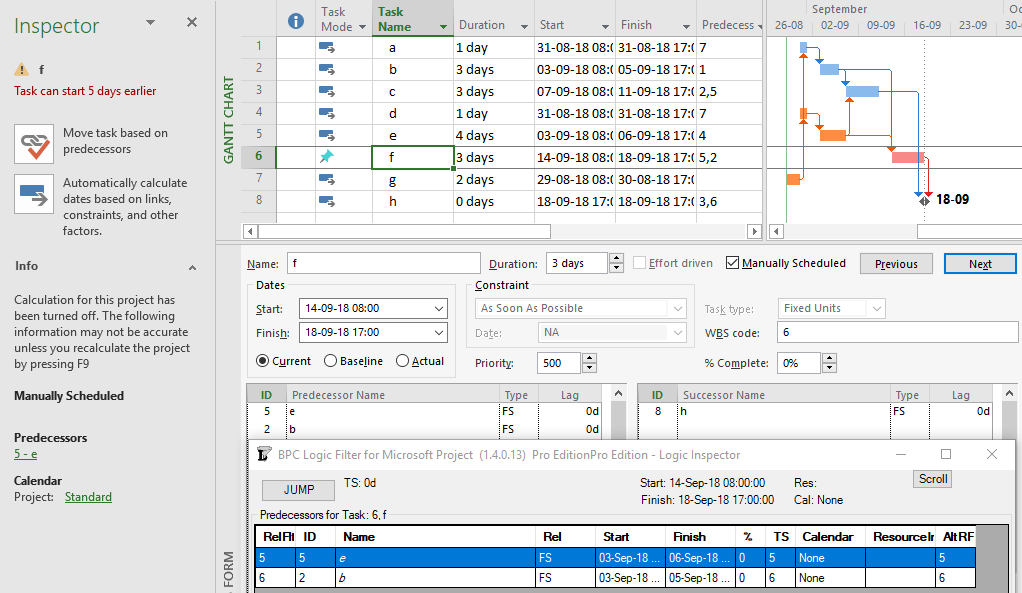
The implicit driving SS relationship from task Sum2 to its outline child task e is correctly identified by the task inspector as well as BPC’s logic inspector.

Those two implicit hierarchical relationships – when combined with the explicit Sum1-to-Sum2 FS relationship – are necessary to properly calculate early and late dates and total slack, which is the source of the critical path depicted.  Unfortunately, the built-in tools are not sufficient to fully trace driving logic through such hierarchical relationships, even in this simple schedule.

Neither summary-task relationships nor the consequent hierarchical (parent/child – child/parent) relationships are explicitly recognized in the generally accepted, traditional understandings of logic-based project scheduling – i.e. the critical path method (CPM) and the precedence diagramming method (PDM).  Such relationships are not generally supported in other scheduling tools, either, so attempts to migrate MSP schedules containing summary logic into other tools for analysis are typically unsuccessful.  It is also clear that adding even a small number of summary-task relationships to a moderately complex project schedule can potentially obfuscate the driving logic paths in the schedule, including the critical path under many circumstances, without fairly sophisticated analysis.  Taking these facts together, most project scheduling professionals seem to agree that summary-task logic in MSP represents poor practice and is to be avoided.

Driving Logic in Backward Scheduled Projects (Microsoft Project)

Microsoft Project’s backward scheduling mode includes numerous traps for novices and professionals alike.  Competent project schedulers avoid it.

In MSP, a backward scheduling mode – sometimes called backward planning, reverse scheduling, or reverse planning – can be invoked by scheduling the project from its finish rather than its start.  In the traditional language of critical path method (CPM) scheduling, it’s most simply described as a late-dates schedule.  Backward planning is useful in several non-standard methodologies, including critical chain project management and the pull planning aspects of the Last Planner System.

The Mechanics of Backward Scheduling

When specified for the active project, this mode essentially does the following:

  1. Sets the default constraint type for all new tasks to as late as possible (ALAP).
  2. Re-sets the constraint type to ALAP for all existing Summary tasks.
  3. [Users choosing this mode in the middle of schedule development must manually re-set the constraint type to ALAP for all existing non-Summary tasks.]
  4. Automatically sets no later than constraints when dates are manually entered into the start or finish fields of tasks.  [Such date entry in forward scheduling mode leads to “no earlier than” constraints, so users choosing this mode in the middle of schedule development should manually review, validate, and potentially re-set any previously-entered date constraints.]
  5. Performs the network scheduling calculations in reverse order, with the reflection point occurring at the project start rather than the project finish.  I.e. the project start date (not the finish, which is user-input) is determined by the logic.
  6. Sets the start and finish of automatically-scheduled tasks to their late dates rather than their early dates.  (This is the most important part.)
  7. Finally, the resource leveling engine resolves resource over-allocations by accelerating higher priority tasks from late dates rather than delaying lower priority tasks from early dates.  Thus, entries in the leveling delay field are negative.  This behavior creates a minor complication regarding use of priority = 1000.  Just as in forward scheduling, a task with priority=1000 is always exempted from any leveling action.  In backward scheduling, this means that priority values of 1000 and 0 are essentially equivalent when considered in the leveling decisions.  The highest effective priority for controlling leveling behavior then becomes 999, not 1000.

Logic relationships used in backward scheduling still have exactly the same meanings that they do in forward scheduling.  A finish-to-start (FS) relationship still means that the two tasks are logically connected such that the successor may not start before the predecessor finishes, and the rarely-applicable start-to-finish (SF) relationship still indicates that it is impossible for the successor to finish before the predecessor starts.  Some users seem to think that backward scheduling involves reversal of these two relationships in particular, but that’s not consistent with the rest of the backward scheduling mode.  Unfortunately, mixing of the two approaches seems to continue, though this typically amounts to invalid date manipulation in my view.

In normal (i.e. forward) scheduling, a task with an ALAP constraint has the dubious distinction of corrupting its entire chain of successors – driving all of them to the critical path.  There are very few legitimate applications for this constraint.  In backward scheduling, the as soon as possible (ASAP) constraint plays a similar role, corrupting its chain of predecessors.  It needs to be avoided in backward scheduling.

When to Use Backward Scheduling

I’ve never used backward scheduling in a real project.  Others have recommended its use to determine the desired start date of a project when the desired completion date is already known.  It also seems consistent, when tasks are suitably buffered, with aspects of critical chain project management that require work to be scheduled as late as possible.

Ultimately, backward scheduling rests on the presumption that tasks can be accelerated (i.e. moved to the left on the bar chart) indefinitely as needed to meet the fixed end date for the project.  Thus, a task whose duration is extended can simply be re-scheduled to start sooner than previously planned, with its predecessors also being accelerated.  Similarly, a higher priority task can be started (and finished) earlier to avoid resource conflicts with a lower-priority task that demands the same resources.  The problem with these presumptions is that time invariably marches forward, and as scheduled dates for incomplete work are overtaken by the vertical time-now line on the bar chart there is no chance for recovery.  The backward scheduling method is pointless if the latest allowable project start date has already been passed – e.g. the project is in progress.

Backward scheduling seems to be of primary value in determining the latest responsible date to start a project (or project segment) while still meeting the desired completion date.  After that latest responsible start date is determined, the project must be converted from backward-scheduled to forward-scheduled mode – manually reviewing and revising the key parameters of each task – if it is to be used for updating and forecasting during project execution.  The original question – i.e. what is the latest responsible project start date? – is just as easily answered by manipulating and examining the late dates of the forward scheduled project.  Thus, for a competent project scheduler, the use of backward scheduling seems largely to be an unproductive diversion.

Driving Logic Analysis

When the logic network is well constructed – and complicating factors like multiple calendars, (early) constraints, and resource leveling are avoided – then the critical path may be reasonably identified by total slack = 0.  Other methods of driving logic analysis must be modified, however.

Under backward scheduling, any slack/float of a task exists on the side towards its predecessors, i.e. to its left on a bar chart.  A driving relationship exists when a successor prevents a predecessor from being scheduled any later than it is.  This means that there are driving successors and driven predecessors.  Consequently, the Longest Path in a backward scheduled project is the driving (successor) path from the project’s start.

MSP includes two built-in methods for reviewing and analyzing driving logic: the Task Inspector pane and the task paths bar styles.  As I wrote in this article a few years ago, I’ve found these tools to be unreliable in complex real-world project schedules.   Under backward scheduling, they are essentially useless and/or misleading.

To start with, Task Inspector simply doesn’t work with backward scheduling.  Opening TI on a backward scheduled project yields the following message:  This project is set to Schedule from Finish.  We are unable to provide scheduling information.

Also under backward scheduling, the Driving Predecessors and Driven Successors bar styles are still derived from Early Dates, as they are in Forward Scheduling.  This makes them essentially useless for assessing the controlling logic of the displayed (late-dates) schedule.  Consider the example below, where all four Task Path bar styles have been imposed, and Task 11 – A2 Structures – is selected.  (The automatic “Slack” bar style is also imposed, but it is invisible since Free Slack – formally defined by Early dates alone – is uniformly zero.)

The selected task is in fact driving/controlling the displayed dates of both of its predecessors (LRF=0), but only one of them displays the correct bar style (the one that, with ERF=0, was the driving predecessor during the forward pass).  Of Task 11’s four successors, only the first (Task 13 – A2 Electrical) is directly driving/controlling Task 11’s schedule, with LRF=0.  The tasks for two of the remaining three successor relationships are incorrectly highlighted, while the third (Task 14) is correctly highlighted only because it is driving/controlling Task 13 – a case of redundant logic.  (All four successors were driven successors during the forward pass.)  Thus in a backward scheduled project, the Task Path bar styles for Driving and Driven dependencies are meaningful (or “correct”) ONLY along the Longest/Critical path of the project, where Early dates and Late dates coincide.  The relationships along that path are driving in both directions; i.e. they are bi-directional driving relationships.

BPC Logic Filter – my company’s Add-In for logic analysis of MSP schedules – identifies driving logic based on relationship free float, which we often call “relative float.”  In BPC Logic Filter, the Longest Path and near-longest paths of simple, backward-scheduled projects can be found using the Task Logic Tracer, starting from the project start milestone and using appropriate settings (i.e. driving relationships in successor direction).  As illustrated in the example project, this is fairly trivial since the results are 100% aligned with Total Slack.

Other driving logic paths (not on the Critical Path) are not so trivial but are easily addressed using BPC Logic Filter, provided that the impact of multiple calendars is minimal.

Precision analysis of more complex, backward-scheduled projects requires some modest modifications to the algorithms.  In particular, several variations of late-relationship-float need to be computed, and these have been added to the development roadmap for the software.

[Apr’20 Revision.  I’ve updated the two figures to incorporate the early-date relative float (ERF) and late-date relative float (LRF) columns in the logic inspector windows.  Calculation of the latter was only added to recent builds of BPC Logic Filter.  These windows also flag the forward-driving (yellow), backward-driving (rose), and bi-directional-driving (red/yellow) relationships.]

What is the Longest Path in a Project Schedule?

In Project schedules, the Longest Path yields the Shortest Time.  Aside from the mental gymnastics needed to digest that phrase, the concept of Longest Path – especially as implemented in current software – has deviated enough from its origins that a different term may be needed.   

Critical Path as Longest Path

Authoritative definitions of the “Critical Path” in project schedules typically employ the words “longest path,” “longest chain,” or “longest sequence” of activities … (that determine the earliest completion date of the project.)  In other words, the path, chain, or sequence with the greatest measured length is the Critical Path.  As a rule, however, none of the associated documents are able to clearly define what constitutes the length of a logic path, nor how such length will be measured and compared in a modern project schedule.  Without a clear standard for measuring the length of something, explicitly defining the Critical Path in terms of the longest anything is just sloppy in my view.

The Original Path Length

Assessing path length used to be much easier.  In the early days of CPM (Critical Path Method) scheduling, any project schedule could be guaranteed to have ALL Finish-to-Start relationships, NO constraints, NO lags or leads, NO calendars, and only ONE Critical Path.  Under these conditions, the length of a logic path could be clearly defined (and measured) as the sum of the durations of its member activities.  Thus, the overall duration of a Project was equal to the “length” (i.e. duration) of its Critical Path, which itself was made up of the durations of its constituent activities.  That result is indicated in the figure below, where the 64-day project length is determined by the durations of the 5 (highlighted) activities on the Critical Path.  Adding up the activity durations along any other path in the schedule results in a corresponding path length that is less than 64-days – i.e. not the “longest” path. [The network diagram was taken from John W. Fondahl’s 1961 paper, “A Non-Computer Approach to the Critical Path Method for the Construction Industry,” which introduced what we now call the Precedence Diagramming Method.  Unfortunately, Microsoft Project (MSP) has an early limit on dates, so his presumed ~1961 dates could not be matched.]

Fortunately, in such simple projects, it’s never been necessary to aggregate and compare the lengths of every logic path to select the “longest path.”  The CPM backward pass calculations already identify that path by the activities with zero-Total Float/Slack, and successively “shorter” paths are identified by successively higher Total Float/Slack values.  This fact has been verified in countless student exercises involving simple project schedule networks, typically concluding with the axiom that “the Critical Path equals the longest path, which equals the path of zero-Total Float/Slack.”

Float/Slack and Path-Length Difficulties

In general, modern complex project schedules have, or can be expected to have, complicating factors that make Total Float/Slack unreliable as an indicator of the Critical Path – e.g. non-Finish-to-Start relationships, various early and late constraints, multiple calendars, and even resource leveling.  See this other article for details.  Therefore, as noted earlier, the axiomatic definition has been shortened to “the Critical Path equals the longest path.”

Unfortunately, finding the “longest path” by arithmetically summing the activity lengths (i.e. durations) along all possible logic paths and comparing the results – not easy to begin with – has gotten more difficult.  Lags, excess calendar non-working time, and resource leveling delays all add to the apparent “length” of a logic path compared to the simple summation of activity durations.  Early date constraints may introduce delays that are not justified by task durations or logic relationships, breaking the path altogether.  On the other hand, leads (negative lags), excess calendar working-time, and the use of overlapping-activity relationships (e.g. SS/FF) reduce its length.  In addition, any hammocks, level-of-effort, and summary activities need to be excluded.  All such factors must be accounted for if the “longest path” is to be established by the implied method of measuring and comparing path lengths in the project schedule.  I don’t know of any mainstream project scheduling software that performs that kind of calculation.  Alternatively, Deep Schedule AnalysisTM using the proprietary HCP (Hidden Critical Path) Method – from HCP Project Management Consulting – appears to compute and compare the lengths of all logic paths in Primavera and MSP schedules.

Longest Path as Driving Path

Contrary to summing up and comparing logic path lengths, most current notions of the “longest path” are based on an approach that does not involve path “length” at all.  As a key attribute, the longest path in a simple, unconstrained and un-progressed project schedule also happens to be the driving logic path from the start of the first project activity to the finish of the last project activity.  It is a “driving logic path” because each relationship in the path is “driving”, that is it prevents its successor from being scheduled any earlier than it is.  Driving relationships are typically identified during the forward-pass CPM calculations.  Subsequently, the driving path to the finish of the last activity can be identified by tracing driving logic backward from that activity, terminating the trace when no driving predecessors are found or the Data Date is reached.  The resulting driving path to project finish is sometimes called the “longest path” even though its “length” has not been established.  This is the “Longest Path” technique that has been applied for nearly two decades by (Oracle) Primavera and adopted more recently in other project scheduling tools.

As of today, MSP continues to define Critical tasks on the basis of Total Slack, but it provides no explicit method for identifying the “Critical Path” using a “longest path” criterion.  How is the responsible MSP scheduler supposed to respond to a demand for the “critical path” when the longest path has been obscured?  Here are several options:

  1. Continue to make simple projects, avoiding all complicating factors like calendars (including resource calendars), early and late constraints, deadlines, and resource leveling. Then assume that “Total Slack = 0” correctly identifies the Critical Path.
  2. If you are using MSP version 2013 or later,
    • Ensure that your project is properly scheduled with logic open-ends only present at a single start and single finish task/milestone, then select the single finish task,
    • Try to use the “Task Path” bar highlighter to highlight the “Driving Predecessors” of your selected finish task.  In the example below, a Deadline (a non-mandatory late-finish constraint) has been applied to task Op12 in the 1961 example, and MSP has responded by applying the “Critical” flag (based on TS=0) to Op12 and its predecessors Op10 and Op2.  As a result, the Critical Path is obscured.  Applying the bar highlighter and selecting task Op18 (the project’s finish task) correctly identifies the driving path to project completion, i.e. the “longest path.”  (For clarity, I manually added the corresponding cell highlighting in the table; the bar highlighter doesn’t do that.)
    • If necessary, create and apply a corresponding filter for the highlighted bars. I’ve posted a set of macros to make and apply the filter automatically in this article.
  3. If you are using MSP version 2007 or later,
    • Ensure that your project is properly scheduled with logic open-ends only present at a single start and single finish task/milestone, then select the single finish task,
    • Try to use the Task Inspector to identify the driving predecessor of the selected task, then go to it and flag it as being part of the driving path. Repeat this until the entire driving path is marked.
    • If necessary, create and apply a filter and/or highlighting bar styles for the flagged tasks.
    • I’ve posted another set of macros to do all this (except bar highlighting) automatically in this other article.
  4. Note: The previous two approaches both rely on MSP’s StartDriver task object to identify driving relationships. As noted in this article, however, the resulting driving logic is not reliable in the presence of tasks with multiple predecessors, non-FS predecessors, or actual progress.
  5. Use BPC Logic Filter or some other appropriate add-in to identify the “longest path” in the schedule.

Whichever method or software is used, expressing the Longest Path using the Driving Path methodology has one key weakness: it has not been proved generally useful for analysis of near-critical paths.  While the Longest Path may be known, its actual length is not readily apparent.  More importantly, there is no generally-accepted basis for computing the lengths, and hence the relative criticality, of the 2nd, 3rd, and 4th etc. Longest Paths.  Consequently, Near-Critical paths continue to be identified based on Total Float/Slack, which is still unreliable, or – in P6 – based on unit-less “Float Paths” from multiple float path analysis.

“Longest Path” and Early Constraints

As noted several times here, the methods described for identifying the “longest path” are in fact describing the “driving path to the project finish.”  This distinction can raise confusion when one or more activities in the project schedule are delayed by an early constraint.  Consider the case below, where an activity on the longest path (Op13) has been delayed 2 days by an early start constraint.  Consequently, its sole predecessor relationship (from Op3) is no longer driving, and Op3 gains 2 days of Total Float/Slack.  As shown by MSP’s “Driving Predecessor” bar highlighter, the driving logic trace is terminated (going backwards) after reaching the constrained task.

Identical results are obtained from Primavera’s (P6) Longest Path algorithm.  This is neither surprising nor incorrect; the project’s completion is in fact driven by the external constraint on Op13, and its predecessor Op3 is quite properly excluded.

In this case, the application of an early constraint on a longest-path task simply truncates the longest path, which may be re-established using a logic tracing routine that jumps the constraint.  In general, however, early date constraints can substantially change the driving path to project completion, such that the length (i.e. aggregate duration) of any particular logic path becomes irrelevant.  For example, the next figure shows the consequences of imposing a one week (external) delay to Task Op11 in lieu of the earlier constraint.  This leads to a 3-day delay of the project’s finish and a shift of the both the driving path and the zero-float path from Task Op13 to Op11.  The total length of the corresponding critical path (including Op11’s formerly-driving predecessors) is 62 days.  The 64-day path leading through Op13 and Op15 still exists, but it now has 3 days of total slack and is no longer driving the project completion.  Thus, the mathematical longest path carries no significance in this constrained project schedule.


It’s clear therefore that the driving path to project completion and the longest path from the project start (or Data Date) to the project completion can differ when early constraints are present.  P6’s “Longest Path” algorithm automatically defaults to the driving path, not the aggregate longest path, and to date there have been no built-in alternatives to that behavior.  As a result, some consultants suggest that P6 Longest Path analyses should be rejected when external constraints – even legitimate ones like arrival dates for Customer Furnished Equipment – are present.  Unfortunately, a position that requires strict duration-summing to identify critical (i.e. “longest”) paths in schedules containing early constraints appears to be both misleading and inconsistent with standard schedule calculating methods.  (A P6 add-in, Schedule Analyzer Software, does claim to provide a true Longest Path representation in the presence of early constraints.)

BPC Logic Filter – Longest Path Filter

BPC Logic Filter is a schedule analysis add-in for MSP that my company developed for internal use.  The Longest Path Filter module is a pre-configured version of the software’s Task Logic Tracer.  The module is specifically configured to identify the project’s longest path (as driving path) through the following actions:

  1. Automatically find the last task (or tasks) in the project schedule.
    • Excluding tasks or milestones that have no logical predecessors. (E.g. completion milestones that are constrained to be scheduled at the end of the project but are not logically tied to the actual execution of the project. The resulting trace would be trivial.)
    • Excluding tasks or milestones that are specifically flagged to be ignored, e.g. (“hammocks”)
  2. Trace the driving logic backwards from the last task to the beginning of the project.
    • Driving logic is robustly identified by direct computation and examination of relative floats. (Driving relationships have zero relative float according to the successor calendar.)  The unreliable StartDriver task objects are ignored.
    • Neither completed nor in-progress tasks are excluded from the trace.
  3. Either apply a filter to show only the driving logic path, or color the bars to view the driving logic path together (in-line) with the non-driving tasks. The example below is identical to the previous one, but BPC Logic Filter formats the bar chart to ignore the impacts of the applied deadline.  The resulting in-line view is substantially identical to the bar chart of the original, unconstrained project schedule. 

BPC Logic Filter and the (True) Longest Path

As noted earlier, even a a single early constraint can truncate the driving path to project completion or change the driving path altogether.  In either case, it is debatable in my view whether the addition of non-driving, float-possessing activities into the “longest path” makes that term itself more or less useful with respect to the typical uses of the “Critical Path” in managing and controlling project performance.  If necessary, it is easy to add such activities – as unconstrained drivers of any constrained task – in BPC Logic Filter by checking a box.  The bar chart below shows the results of the Longest Path Filter on the first early-constrained example schedule, as set up according to the driving-path (Primavera) standard.  Results are identical to those of the built-in “Driving Predecessors” highlighter in MSP (above) and of P6.

The next chart shows the complete “longest path” for the project, including the non-driving Op3 activity.

The second chart is different because the check box for “Override if successor task is delayed by constraint” has been checked in the analysis parameters form.  Checking the box causes the non-driving predecessor with the least relative float to be treated as driving, and therefore included in the Longest Path, in the event of a constraint-caused delay.

For a quick illustration, see Video – Find the Longest Path in Microsoft Project Using BPC Logic Filter.

BPC Logic Filter and Near Longest Paths

As noted earlier, the normal methods for identifying the “longest path” (i.e. the driving path) in a project schedule have not been generally adopted for analyzing near-longest paths.  P6 offers multiple float path analysis, which I wrote about here.  In addition,  Schedule Analyzer (the P6 add-in mentioned earlier) computes what it calls the “Longest Path Value” for each activity in the schedule – this is the number of days an activity is away from being on the Longest Path (i.e. the driving path to project completion.)   In the absence of demonstrated user demand, however, MSP seems unlikely to gain much beyond the Task Path bar highlighters.

BPC Logic Filter routinely computes and aggregates relative float to identify driving and near-driving logic paths in MSP project schedules.  In this context, “near-driving” is quantified in terms of path relative float, i.e. days away from driving a particular end task (or days away from being driven by a particular start task.)  Its “Longest Path” and “Near Longest Path” analyses are special cases where the automatically-selected end task is the last task in the project.  For the Near Longest Path Filter, tasks can be shown in-line (with bar coloring) or grouped and sorted based on path relative float.  The “override if successor is delayed by constraint” setting has no effect when the Near Longest Path Filter is generated.  In that case, the non-driving task will be displayed according to its actual relative float.  For example Op3 is shown below with a relative float of 2 days (its true value), not 0 days as shown on the earlier Longest Path Filter view.

Recap

  1. In the development of the Critical Path Method, the “longest path” originated as one of several defining characteristics of the “Critical Path” in simple project schedules. Specifically, the “Critical Path” included the sequence of activities with the highest aggregated duration – i.e. the “longest path”.  Actual computation and comparison of path lengths was not necessary since relative path lengths could be inferred directly from Total Float – a much easier calculation.
  2. Complicating factors in modern project schedule networks tend to confuse the interpretation of Total Float, such that it is no longer a reliable surrogate for path length. As a result, the most recent, authoritative definitions of the Critical Path tend to omit references to float while retaining references to “longest path” and, typically, logical control of the project completion date.  [Notably, the measurement and comparison of aggregated path durations (path lengths) has not been an explicit feature of any mainstream project scheduling tool, so the “longest-path” part of the definition cannot be definitively tested in general practice.]
  3. Notions of “longest-path” among current schedule practitioners are heavily influenced by the deceptively-named “Longest Path” feature in Oracle/Primavera’s P6 software. Perversely, that feature DOES NOT aggregate activity durations along any logic paths.  Rather, it identifies the driving/controlling logic path to the project’s early finish date.
  4. The “Longest Path” in P6 (i.e. the Driving Path to Project Completion) and the “longest path” (i.e. the logic path with highest aggregated duration) are NOT equivalent, particularly when the “Longest Path” is constrained by an early date constraint. There is at least one P6 add-in claiming to identify the true “longest path” (and near-“longest paths”) in this case.
  5. Microsoft Project provides several inefficient methods to identify the Driving Path to Project Completion in simple projects, but these methods are not reliable in the presence of non- Finish-to-Start relationships. There are no native MSP methods for identifying near-driving tasks nor the true “longest path” in the presence of early date constraints.  BPC Logic Filter is an MSP add-in that automatically fills these gaps.
  6. As conceived, the “longest path” criterion implied the transparent calculation and comparison of aggregated activity durations along each logic path in a project schedule. As for Total Float, however, such calculations in complex schedules have been obfuscated by complications like non- Finish-to-Start relationships, lags, and multiple calendars.  Since such obfuscation makes path lengths essentially un-testable, it appears that future Critical Path definitions should omit the “longest path” criterion in favor of a simple “driving path to project completion.”

Longest Paths in Backward Scheduled Projects (MSP) [Jan’19 Edit]

As pointed out in this recent article, the Longest Path in a backward scheduled project is essentially the “driven path from the project start,” not the “driving path to project completion.”

For more information, see the following links:

Article – Tracing Near Longest Paths with BPC Logic Filter

Video – Analyze the Near-Longest Paths in Microsoft Project using BPC Logic Filter


Problems with Driving Logic in Task Inspector and Task Paths (Microsoft Project 2010-2016)

Neither the Task Inspector nor the “Task Path” bar highlighter is a reliable indicator of task driving logic in Microsoft Project in the presence of mixed-type predecessor relationships or Backward Scheduling. 

At first glance, the Task Inspector pane in Microsoft Project (MSP) seems to be a reasonable tool for revealing the logic that is largely hidden in project schedules.  After all, you just select a task, click “Inspect Task”, and MSP provides a hyperlinked list of “Predecessor Tasks” that are controlling the schedule dates of the selected task.  For simple (i.e. Finish-to-Start) relationships between tasks with no progress, this assumption seems generally correct.

Unfortunately, many times Task Inspector is just plain wrong. (The examples below are taken from a ~1000-task real-world project schedule with actual progress updates.  Task names were obfuscated for confidentiality).  Each example represents many more cases in the schedule.

1. Once an actual start is recorded, logical drivers constraining the finish are ignored.

2. In case of parallel FS and SS driving predecessors, the FS driver is ignored.

Here is the corresponding bar highlighting from Task Path’s Driving Predecessors (MSP 2016).  The noted red bar should be orange like the one below it.

3. In case of parallel FS and FF driving predecessors, the FF driver is ignored.

3. In some (but not all) cases, an FF predecessor with substantial relative float is identified as the driving predecessor, while the true FS driver is ignored.

In general, the issues are present mainly in tasks with multiple predecessors of different types.  In forward scheduled projects, they are not found in un-started tasks whose predecessors are all of type Finish-to-Start.

The “Driving Predecessors” bar highlighter of the Task Path tool in Microsoft Project Professional 2016 has the same issues as the Task Inspector results shown here.  They are both consistent with the StartDriver object for each task.  Any driving-logic tracer based on the StartDriver object – including those provided in my blog (Macro for Listing Driving Predecessors and QuickTrace Macros ) – has similar issues.

In the examples above, the task predecessors are displayed in Logic Inspector views from BPC Logic Filter (our MSP Add-in).  Predecessors are “driving” if their relative floats are zero; i.e. there is no working time between the corresponding predecessor and successor dates.  The driving predecessors identified in the examples are easily confirmed by examining the dates.  [Though illustrated mostly using Microsoft Project Professional 2010, all examples have been confirmed in Microsoft Project Professional 2016.]

Though not really highlighted here, it bears noting that MSP’s “driving logic” indicators are completely oblivious to resource-leveling decisions.  Thus, resource-driving logic is not addressed.  In contrast, BPC Logic Filter handles resource-driving logic quite well.

On Manually Scheduled Tasks [Aug’18 Edit]

If a manually scheduled task has predecessors, then MSP will identify one or more of them as the driving predecessor even when the manual scheduling has substantially delayed the task compared to the logic requirements.  This is one of the few factors differentiating a manually scheduled task from a normal (i.e. automatically scheduled) task with a mandatory constraint.  In this case, the Task Path “Driving Predecessors” bar highlighter ignores the delay and continues to trace “driving” logic through the identified start drivers.  (The Task Inspector suggests that the user either accelerate the task to remove the delay or convert the task to automatic scheduling.)  As a consequence, a schedule with manually scheduled tasks can have a driving path to project completion (according to Task Path) that is substantially different from the Critical Path that is based on Total Slack.

In Backward Scheduled Projects [Jan’19 Edit]

As pointed out in this recent article, neither the Task Inspector nor Task Path bar styles are useful in backward scheduled projects.