Overlapping Tasks in Project Schedules

In a project schedule, overlapping tasks are tasks that are BOTH sequential and concurrent.  The effective and efficient scheduling of overlapping tasks typically requires the use of time lags and logic relationships that are not Finish-to-Start.

Introduction

In a project schedule, overlapping tasks are tasks that are BOTH sequential and concurrent, with neither condition being absolute.  They can exist in highly-detailed schedules for project engineering, design, production, and construction, though they are much more common in high-level summary schedules.  Essentially, Task A and Task B are overlapping when:

  1. Task B is a logical successor of Task A; and
  2. Task B can start before Task A is finished.

Handling the second condition typically requires the use of time lags and logic relationships that are not Finish-to-Start.  These elements were not supported in the original Critical Path Method (CPM), and some scheduling guidelines and specifications still prohibit or discourage their use.  Nevertheless, they remain the most effective tools for accurately modeling the plan of work in many cases.

There are essentially two categories of overlapping task relationships: Finish-Start Transitions and Progressive-Feeds.

Finish to Start Transitions

Overlapping tasks with Finish-Start Transition relationships can be described in terms of a relay (foot)race, where an exchange zone for handing over the baton exists between each pair of “legs” (i.e. the 4 stages of the race).  At the end of Leg 1, Runner 2 must start running before Runner 1 arrives, timing his acceleration to ensure an in-stride passing of the baton in the exchange zone, simultaneous with the completion of Leg 1.  Runner 2 does not care about Runner 1’s fast start nor his awkward stumble at the midway point; his only focus is on gauging Runner 1’s finishing speed and starting his own run at the precise instant necessary to match speeds in the transition zone.  In practice, Runner 2 establishes a mark on the track – paced backward from the exchange zone – and starts his own run when Runner 1 reaches the mark.

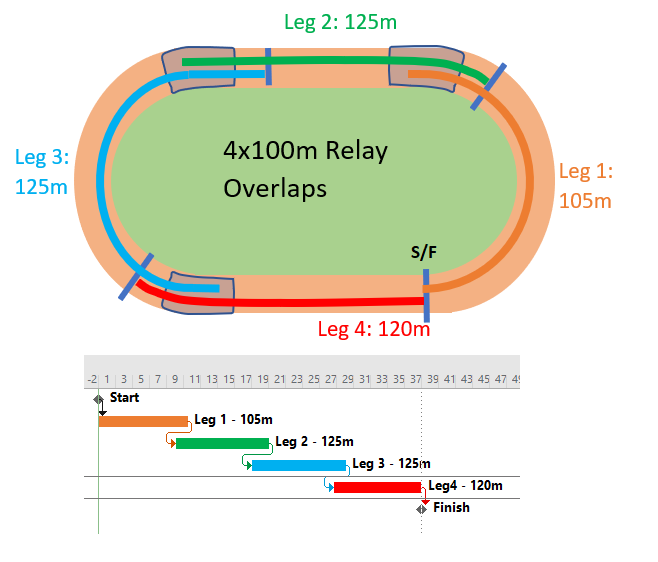
Real-world examples of such overlap include the cleanup/de-mob and mob/setup stages of sequential tasks in construction projects.  In engineering/design, many follow-on tasks may be allowed to proceed after key design attributes are “frozen” at some point near the finish of the predecessor task.  In general, the possibility of modest overlap exists at many Finish-Start relationships in detailed project schedules, sometimes being implemented as part of a fast-tracking exercise.  The most common front-end planning occurrence of these relationship in my experience is in logic driven summary schedules, where analysis of the underlying detailed logic indicates that the start of a successor summary activity is closely associated with, but before, the approaching finish of its summary predecessor.

In terms of a project schedule, this kind of relationship is most easily modeled as Finish-to-Start with a negative lag (aka “lead”).  This is illustrated by the simple project below, where tasks A, B, and C are sequentially performed between Start and Finish milestones.  Each task has a duration of 9 days to complete 90 production-units of work.  (A linear production model is shown for simplicity.)  Because of the Finish-Start Transition, Task B and Task C are allowed to start 1 day before their predecessor finishes. 

Negative lags can be used for date manipulation, such as to hide an apparent delay.  Negative lags can also be the source of float (and critical path) complications for project schedules with updated progress, particularly when the lag spans the data date.  Consequently, negative lags are discouraged or explicitly prohibited in many schedule standards and specifications.

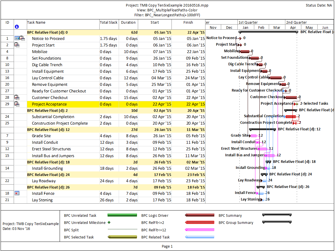
When negative lags are prohibited, overlapping tasks with Finish-Start transitions may be modeled by breaking the tasks into smaller, more detailed ones – all connected with simple Finish-Start links and no lags.  In the example, the two negative-lag relationships can be replaced by two pairs of concurrent 1-day tasks – the last part of the predecessor and the first part of the successor – that are integrated with FS links.  Thus, the overlapping linear production of the three tasks now requires 7 tasks and 8 relationships to model, rather than the original 3 tasks and 2 relationships.  Alternately, each pair of concurrent tasks could be combined into a single “Transition” task, though such an approach could involve additional complication if resource loading is required.

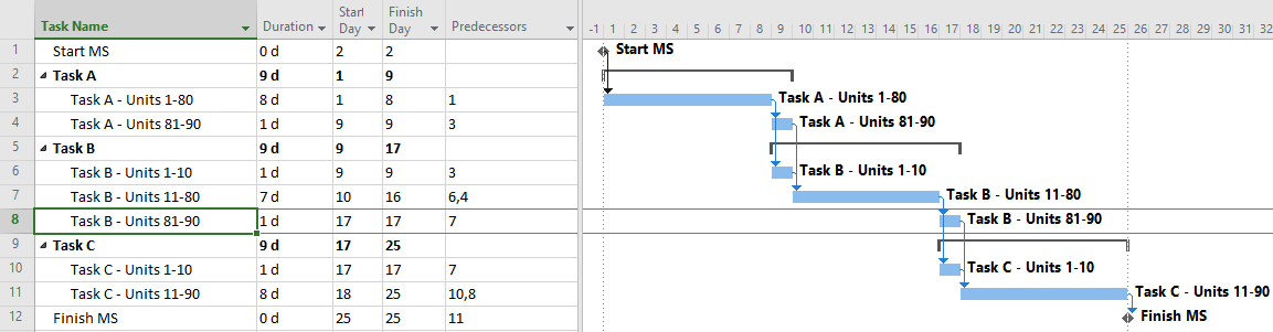
In practice, the extra detail seems hardly worth the trouble for most schedulers, so simply ignoring the overlap seems fairly common.  This has the consequence of extending the schedule.

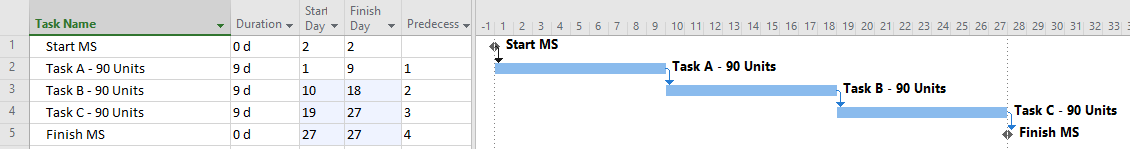
By ignoring the overlap, the scheduler here has added two days (of padding/buffer/contingency) to his overall schedule, extending the duration from 25 to 27 days.  This is unlikely to be recovered.

Overlapping Tasks with Progressive Feeds

The predominant category of overlapping tasks involves repetition of sequentially-related activities over a large area, distance, or other normalized unit of production.  The activities proceed largely in parallel, with the sequential relationships based on progressive feeding of workfront access or work-in-process units from predecessor to successor.  In construction, a simple example might include digging 1,000 meters of trench, laying 1,000 meters of pipe in the trench, and covering the trench.  The most timely and profitable approach to the work is to execute the three tasks in parallel while providing adequate work space between the three crews whose production rates are well matched.  This is often described as a “linear scheduling” problem; common examples in construction are railways, roadways, pipelines, wharves, industrial facilities, and even buildings (e.g. office towers – where steel, concrete, mechanical, plumbing, electrical, finishing, and trim activities need to be repeated for each floor.)  Many large-scale production/manufacturing operations are set up to maximize overall throughput by optimizing the progressive feeding of production units through the various value-adding activities.  Proper scheduling of such activities is necessary when similar techniques are applied in non-manufacturing industries like construction, e.g. production lines for precast concrete piles or panels.

Below is a simple table and associated linear production chart summarizing three sequential tasks (A, B, and C) that must be repeated 90 times along a workfront to complete a specified phase of work.  Each task can be executed 10 times per day, resulting in a 9-day duration for the required 90 units of production.  For safety and productivity reasons, it is necessary to maintain a minimum physical separation of 30 units (i.e. 3 days’ work) between the tasks at all times.  Thus, Task B must not be allowed to start until Task A has completed 30 units of production (~3 days after starting), and it must not be allowed to complete more than 60 units of production (~3 days from finishing) until Task A has finished.  Task C must be similarly restrained with respect to Task B.  As a result, the overall duration of the three tasks is 15 days.

The three tasks must now be incorporated into a logic-based project schedule model.  When doing so, the following potential issues should be kept in mind:

  • In most scheduling tools, relationship lags are based on an implied equivalence between production volume (or workfront advancement) and time spent on the task. The validity of the lags needs to be confirmed at each schedule revision or progress update.  (One exception, Spider Project, may offer more valid methods.)
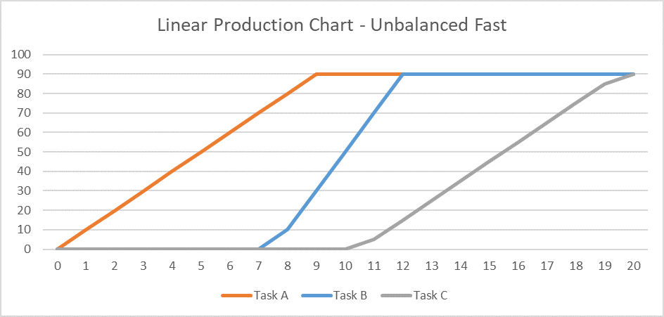
  • Using progressive-feed assumptions with unbalanced production rates can have unintended consequences. For example, if the production rate of Task B is doubled such that the task can be completed in half the time, then the start of the task may be delayed to meet the finish restraint.  This is consistent with a line-of-balance planning philosophy that places the highest priority on the efficient use of resources, such that scarce or expensive resources will not be deployed until there is some assurance that the work may proceed from start to finish at the optimum production rate, without interruption.  In the example, the delayed start of Task B also delays the start of Task C, leading to an increase in the overall project duration from 15 days to 20 days.  Some writers refer to this phenomenon as “Lag Drag.”  The overall schedule is optimized when progressive-feed tasks are managed to the same balanced production rate, and disruptions are minimized.
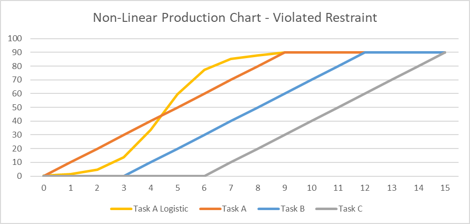
  • A progressive-feed model may not be valid if the physical or temporal requirements underlying the lags at task Start and Finish are violated during task execution. For example, if the daily production rate of Task A follows a classic S-curve profile (“Task A Logistic”) while Task B’s stays linear, then maintaining the required 30-unit minimum physical separation may require additional delay at the start of the second task.

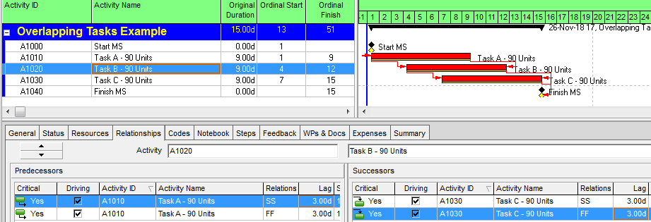
Compound Relationships: The Typical Approach in Oracle Primavera P6

As shown in the following figure, scheduling these overlapping tasks is fairly straightforward in P6.  Because P6 supports multiple relationships between a single pair of tasks, it is possible to implement the required Start and Finish Separations as combined Start-Start and Finish-Finish relationships, each with a 3-day lag.  These are also called “Compound Relationships.”  The resulting representation of the linear schedule is completed with 3 tasks and 4 relationships (excluding the Start and Finish milestones.)  The three tasks are likely well aligned with the labor and cost estimates for the project, so resource and cost loading of the schedule should be straightforward.  The scheduler must still ensure that the three concerns above are addressed, namely: validating lag equivalence to work volumes or workfront advancement, balancing of production rates, and confirming lag adequacy when used with differing task production profiles.

One-sided Relationships: The Typical Approach in MSP

Microsoft Project does not permit more than one relationship between any two tasks in a project schedule (see Ladder Logic in Microsoft Project).  As a result, the scheduler in MSP will typically choose to implement either a Start-to-Start or Finish-to-Finish restraint with a corresponding lag.  Both options are shown in the following figure.

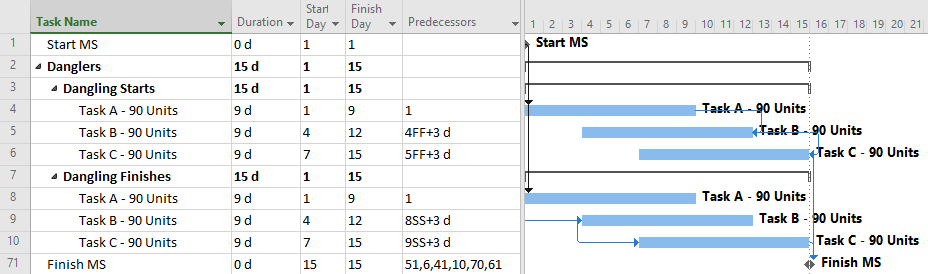
In either case, the resulting schedule will have the lowest number of tasks {3} and relationships {2} to manage (for both cost and schedule) through the project.  This approach is easy to implement.

The most obvious problem with this typical approach is the inadequate logic associated with the dangling starts and dangling finishes (Dangling Logic).  As a result, the typical CPM metrics of Slack (i.e. Float) and identification of the Critical Path will not be reliable, especially after the start of progress updates.

PDM with Dummy Start Milestones

Correcting the dangling logic issues in MSP schedules is most simply addressed using dummy milestones to carry either the start or finish side of the logic flow.  Below I’ve shown two variations using dummy Start milestones:

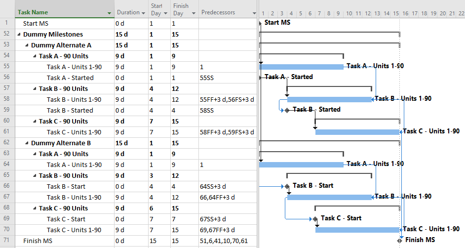
Alternate A involves trailing start milestones.  Here, the milestones exist as start-to-start successors of the corresponding tasks, effectively inheriting their dates from the corresponding task start dates.  The trailing start milestones pass logic to the successor tasks via relationships of the form, start-to-start-plus-lag.

Alternate B involves leading start milestones.  Here the milestones exist as start-to-start successors of the preceding tasks (plus lags) and as start-to-start predecessors of their corresponding tasks (no lags).

The two alternates are largely equivalent, though Alternate B (leading start milestones) has one significant advantage: it works with percentage lags.  When a percentage lag is imposed, the imposed time lag increases or decreases as the predecessor’s duration increases or decreases.  This reduces some of the risks of the assumed production volume = time equivalence.  (Be careful, though; the imposed lag is always a percentage of the overall Duration of the predecessor task, having nothing to do with the Actual (i.e. to-date) Duration.  Moreover, all lags in MSP are imposed using the successor-task’s calendar, so mis-matched predecessor and successor calendars can bring surprises.)

Using the dummy milestones leads to valid schedule logic with a relatively modest addition of detail (i.e. medium number of tasks {5} and relationships {6}.)  The schedule stays fully aligned with labor/cost estimates; no deconstruction is required, and it responds well to unbalanced and varying production rates.  Unfortunately, the dummy milestones can cause visual clutter, so presentation layouts need filters to remove them from view.

Full-Detail: the CPM Ideal

Non-finish-to-start relationships were not supported in the original CPM, and they are discouraged or prohibited in some scheduling standards and specifications.

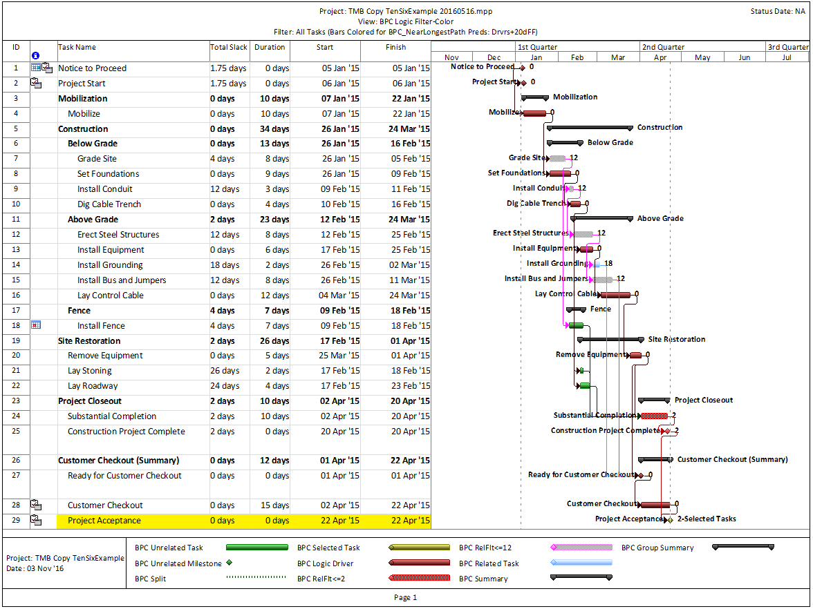
If only finish-to-start relationships are allowed, then accurate modeling of the three overlapping tasks requires substantial deconstruction into a larger number of detailed subtasks.  For the three-task example, the schedule model below breaks each 9-day task into nine 1-day tasks, all integrated with finish-to-start relationships.  The model is depicted using MSP; a similar model could be constructed in P6.

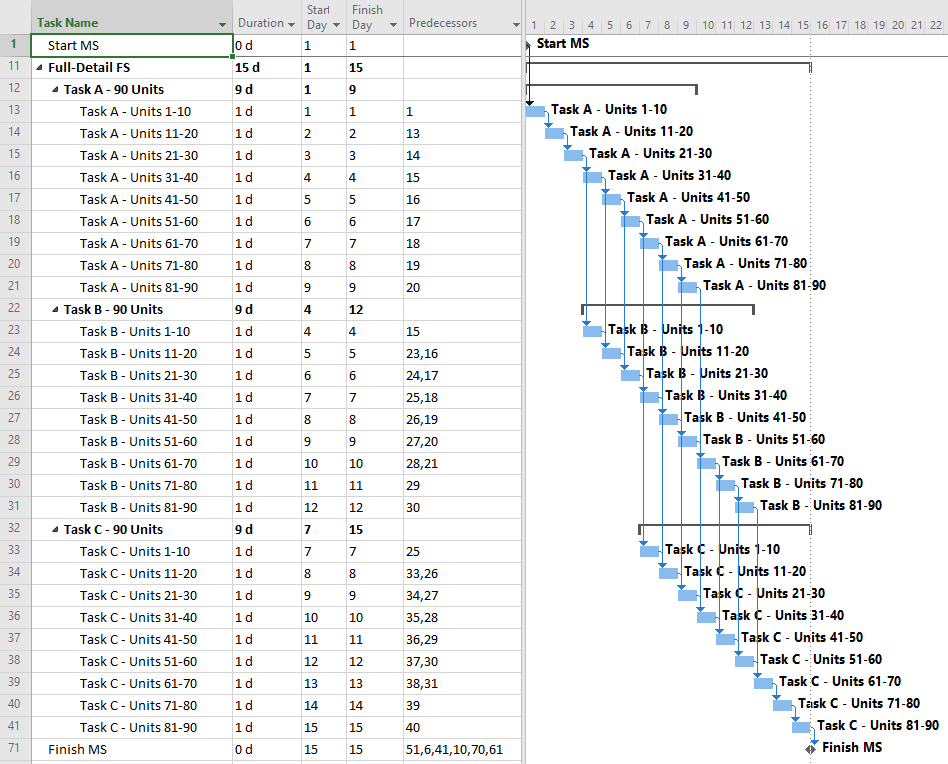
Overall, this approach appears to be more “valid” with respect to pure schedule logic.  That is, there are no leads, no lags, and no non-finish-to-start relationships.  The resulting model can also respond well to unbalanced and varying production rates, and it is likely to stay valid through progress updates.

On the “con” side, this model has the maximum level of detail (i.e. highest number of tasks {27} and relationships {39}.)  Consequently, it will introduce substantial complications to resource and cost loading, and it will be the hardest to manage through completion.  More importantly, the logic relationships that accompany such additional detail are not always technologically required.  While the ordering of Units 21-30 prior to Units 31-40 may appear perfectly reasonable in the office, all that really matters is that ten units of production are received, completed, and passed on to the next task each day.  The addition of such (essentially) preferential logic increases the chances that the actual work deviates substantially from the plan, as field conditions may dictate.  That can severely complicate the updating of the schedule, with no corresponding value added.

Compromise: PDM with Partial Detail

The next figure presents a compromise, providing additional task details as needed to address the initial separation requirements but minimizing the use of lags and non-finish-start relationships.  The result is a moderate schedule with “mostly valid” logic and only modest level of detail (i.e. medium number of tasks {6} and relationships {7}.)  Such a schedule presents medium difficulty of implementation and is less susceptible to the “preferred logic” traps identified earlier.  It also responds well to unbalanced and varying production rates, and it stays valid (mostly) during progress updating.

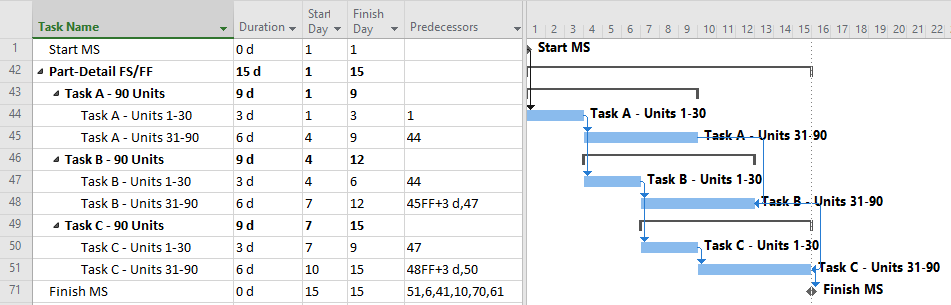
This schedule still requires consideration and validation of the progressive-feed assumptions.  Since this schedule is only partly aligned with existing labor/cost estimates, some de-construction of those estimates may be required for resource and cost loading.

AACE International Annual Meeting 2017

June of 2017 marked my first attendance at the Annual Meeting of AACE International (formerly Association for the Advancement of Cost Engineering). It was in Orlando – kind of a bummer since I had just attended the Construction CPM Conference in Orlando back in January.

Attendees were treated to two excellent keynote addresses: On Monday, Frank Abagnale gave lessons learned from his early life as a globe-trotting teen criminal followed by 42 years in the FBI.  (Leonardo DiCaprio played Abagnale in Catch Me if You Can .)  On Tuesday, Justin Newton of Walt Disney Imagineering gave an excellent presentation on the use of Cost and Schedule controls in constructing Disney’s latest attractions.

The technical sessions were first-rate, and I was continually facing the need to decide between multiple sessions of major interest that were taking place at the same time.  In sum, I wound up participating in four sessions on project risk analysis, two sessions on advanced forensic schedule analysis, and three sessions on advanced planning and scheduling topics.  I also sat in on Dr. Dan Patterson’s showcase of his latest AI-assisted, “knowledge-driven planning” effort, called Basis.   Judging from Dan’s previous successes with Pertmaster and Acumen Fuse/360/Risk, Basis is going to take project management to a whole new level. Finally, I participated in a very robust business meeting of AACE’s Planning and Scheduling Subcommittee.

Besides participating as a regular member of the association, I presented two papers in the Planning and Scheduling Technical Program.  The first is a paper I wrote to address the deduction of resource-driving links in BPC Logic Filter(PS-2413) Extracting the Resource-Constrained Critical/Longest Path from a Leveled Schedule. 

The second is one where I made only a modest contribution in review but agreed to present the paper on behalf of the primary authors who were unable to attend the meeting:  (PS-2670) Draft Recommended Practice No. 92R-17 – Analyzing Near-Critical Paths.

The resulting discussions were stimulating, but judging from the quantitative scoring (based on the speaker evaluation cards), there’s some room for improvement in communicating with this audience.  Lessons learned: 1) Despite the refereed papers, this is not an academic meeting.  Most attendees are seeking professional development (i.e. training) hours on familiar subjects.  Presenting on an esoteric subject like the first paper  – especially one without means of direct application in the prevailing software – is guaranteed to disappoint some; 2) When someone asks you to present their word-choked slide deck on a subject that you don’t completely own – especially a prescriptive procedure like the draft RP – don’t do it.  Nobody will be happy with the result.

I look forward to returning to the annual meeting in 2019.


Video – Using BPC Logic Filter to Analyze Resource-Leveled Critical Path

Here’s another video of BPC Logic Filter in action – this time revisiting the themes of  previous blog entry:  The Resource Critical Path


Tracing Near Longest Paths with BPC Logic Filter

This article highlights the creation of a new targeted report from BPC Logic Filter to identify the “Near Longest Paths” of a project.

While BPC Logic Filter was originally developed as a pure logic tracer, I added a few targeted reports early on to reflect some specific needs, including the “Longest Path Filter” and the “Local Network Filter.”  This article highlights the creation of a new targeted report to identify the “Near Longest Paths” of a project.

Often, when presented with a new project schedule in Microsoft Project, my first step (in concert with a logic health check) has been to run a Longest Path Filter analysis using BPC Logic Filter.  This report quickly and clearly identifies the driving path to project completion.  While the resulting filtered task list is useful for reporting, it rarely satisfies the needs of a serious analysis.  The second step, therefore, is to identify the associated near-longest-paths of the project by running a “Task Logic Tracer” predecessor analysis – with a positive relative float limit – for the project completion task.  The result is a clear description of the driving and near-driving paths to project completion.  The latest release of BPC Logic Filter adds a specific command to combine these two actions and generate a single “Near Longest Path Filter” for the project.

The mechanics are pretty simple.  As usual – with a Gantt view active in a project that contains logic – just open the Add-Ins ribbon [changed to the BPC ribbon in subsequent versions] and click on the button for “Near Longest Path Filter.”

bpclogicfilter-ribbongroup1611

The add-in will initialize, and the user is given a choice of modifying the default analysis parameters.  Some of the parameters are pre-set and can’t be changed here.  The key parameter for a formal Near-Longest-Path analysis is the Relative Float Limit, highlighted below.  Any related task with a Path Relative Float that is less than the specified limit will be included in the filter; all others will be ignored and considered unrelated.  The default value is 100 days away from the driving/longest path (which can be changed in the Settings).

bpclogicfilter-near-longest-path-window

The standard output for a simple project (using the parameters selected above) is provided here.  Selecting “Re-Color Bars” instructs the add-in to generate the custom output shown, including the header, the legend, and five different bar colors depending on proximity to the Longest Path.  Thresholds for applying these bar colors can be manually adjusted in the program settings or, if desired, automatically adjusted by the add-in.  nlp_tensixexampleltr

Here’s an alternate view showing the Near Longest Paths in-line in the context of an existing Outline/WBS organization.  In this analysis I reduced the Relative Float Limit from 100 to 20 days, and the three tasks at the bottom of the earlier figure were ignored.  Here they are given a green “BPC Unrelated Task” bar.

nlp_tensixexampleinlineltr

While I’ve always hated redundant work, this particular improvement to BPC Logic Filter was kick-started by my recent review of the draft of “Analyzing Near-Critical Paths,” a pending Recommended Practice from AACE International.  The new draft recommended practice is based largely on the previously-published (2010) Recommended Practice 49R-06 – Identifying the Critical Path.  According to both documents, Critical- and Near-Critical paths may be identified on the basis of total float/slack thresholds (in the absence of variable calendars, constraints, or other complicating factors) and – when total float/slack does not suffice – “closeness to the longest path.”  For the latter cases, 49R-06 suggests two methods of analysis:

  • Longest Path Value – a metric that appears similar to Path Relative Float (in BPC Logic Filter) for the project completion task. This metric has been applied as an add-on to Oracle Primavera scheduling tools: See Ron Winter’s Schedule Analyzer.
  • Multiple Float Path analysis. Like the Longest Path Value, Multiple Float Path analysis is primarily associated with Oracle’s Primavera scheduling tools – it is presented as an advanced scheduling option in P6.  As I’ve noted in Beyond the Critical Path – multiple float path analysis indicates closeness to the longest path without explicitly measuring and presenting it.  Detailed examination of the results, including relationship free floats, is necessary to determine the apparent relative float of each activity.

From its start, BPC Logic Filter has supported a similar analysis for Microsoft Project schedules through its Path Relative Float metric, Multiple-Float-Paths views, and other reporting.  The new “Near Longest Path Filter” offers a single-step approach to identifying and analyzing near-critical paths in the presence of variable calendars, constraints, and other complicating factors – when Total Slack becomes unreliable as an indicator of logical significance.

See also Video:

Video – Analyze the Near-Longest Paths in Microsoft Project using BPC Logic Filter


Float is not Schedule Contingency, Except when it is

I am writing this as a reminder to myself and to colleagues.

Total Float is NOT schedule contingency.  That’s right: Total Float is NOT schedule contingency.  I say this after the umpteenth conversation with a very smart and experienced contractor who regularly uses the terms interchangeably.

First, a couple references:

Merriam-Webster

Merriam-Webster defines “contingency” as a Noun thus:

1a contingent event or condition: such as

aan event (such as an emergency) that may but is not certain to occur

bsomething liable to happen as an adjunct to or result of something else 

2the quality or state of being contingent

When budgeting projects, our usage of the term has evolved from an “allowance for contingencies”, through “contingency account”, to often a simple “contingency” amount – setting aside funds for uncertain costs or unknown risks in project scopes.  Similarly, a “schedule contingency” exists as an explicit setting-aside of time to address uncertain durations or risks in project schedules.

AACE

AACE International (formerly the Association for the Advancement of Cost Engineering International) issued a Recommended Practice for Schedule Contingency Management (70R-12) that defines schedule contingency as, “an amount of time included in the project or program schedule to mitigate (dampen/buffer) the effects of risks or uncertainties identified or associated with specific elements of the project schedule.”  Then the RP emphasizes, “Schedule contingency is not float (i.e. neither project float* nor total float).”  Finally, the RP goes on to define Project Float (in a footnote) as, “the length of time between the contractor’s forecast early completion and the contract required completion.”  A key theme of the recommended practice is to make schedule buffers explicit, visible, and allocated to specifically identified schedule risks.

* I might quibble with the “project float” exclusion, particularly in any case where risk mitigation is its primary motivation.

ASCE

The American Society of Civil Engineers recently published a new standard:  ANSI/ASCE/CI 67-17 – Schedule Delay Analysis.  Page 5 of this new standard provides a fairly long definition of “Float” that seems essentially correct with the pronounced exception of its first clause, “Float — The time contingency that exists on a path of activities.”  Obviously, this is a direct contradiction to the AACE definition above.  It also appears largely at odds with the rest of the definition in the ASCE standard.

DCMA

The Defense Contract Management Agency (DCMA) promulgated a 14-Point Assessment methodology for analysis of Integrated Master Schedules, which seems to have been widely adopted in some industries.

Point 13 of the DCMA’s 14-Point Analysis defines the Critical Path Length Index (CPLI) as:

                Critical Path Length + Total Float

CPLI  =   ____________________________________

                       Critical Path Length

Here the “Critical Path Length” is essentially the time (in days) from the current data/status date until the forecast completion date of the project.  The “Total Float” used in the ratio turns out to be the difference between the forecast completion date and the baseline/contract completion date – we otherwise know this as “Project Float.”  (This is also the value of Total Float that Oracle’s Primavera P6 scheduling software displays on the Critical Path when a Project “must finish by” constraint corresponding to the contract completion date is assigned.)

The DCMA guidance provides a target value of 1.00, corresponding to a Project Float of 0.   It goes on to suggest that a CPLI greater than 1.00 (i.e. Project Float is positive) is favorable while a CPLI less than 1.00 (i.e. Project Float is negative) is unfavorable.

NEC ECC

The NEC Engineering and Construction Contract (ECC), a collaborative contract form with increasing use in UK and Commonwealth countries, has formalized the use of two alternate terms for schedule contingencies:

Terminal Float

Terminal Float is the difference between the current Planned Completion date and the (Contract) Completion Date.  It is not of a fixed size, is not allocated to any particular risk(s), and is reserved for the exclusive use of the Contractor.  Notably, an acceleration of early activities that results in acceleration of the Planned Completion date also increases the Terminal Float.  Terminal Float is equivalent to the Project Float of AACE International terminology.

Time Risk Allowance

Time Risk Allowance (TRA) “is made by the contractor when preparing its programme. These are owned by the contractor and provided to demonstrate that the contractor has made due allowance for risks which are the contractor’s under the contract.  They must be realistic – unrealistic allowances could prevent the project manager from accepting the programme.”  In other words, TRA is explicit time contingency buffer/allowance that is allocated to specific activities and risk events in the project schedule.

Clause 31 of the NEC Engineering and Construction Contract (ECC) requires the Contractor to show float and “time risk allowance” (TRA) on the programme (i.e. schedule).  The NEC does not specify exactly how to “show” the TRA, though the demand that it be “realistic” has been used to justify a requirement that TRA be distributed through the project schedule based on explicit risk assessment (like the AACE RP).  Typically, the TRA is included in padded activity durations, with the specific TRA portion explicitly noted in a custom field for each activity.  In any case, the TRA participates directly (as a duration) in the CPM calculations for the deterministic project schedule, an output of which is Float.  (Obviously, it must be excluded from any schedule risk simulations.)

Confusion

The mixed definitions have led to some confusion and contradictory recommendations from professionals.

The ASCE document on Schedule Delay Analysis implies that “time contingency” simply exists, manifested as Float, on a network path.  This is far from the common use of “contingency” as an explicit and proactive allowance for risk.

In the NEC environment, there seems to be a persistent tendency to conflate TRA with various types of Float, with some reputable legal sources describing both Terminal Float and “Activity” float as “leeway the contractor adds” in case of problems.  In some cases, contractors are being advised to explicitly mis-identify activity Free Float as Time Risk Allowance in their project schedules, thereby reserving that portion of the activity’s Total Float for themselves.

My View:

Total Float and its components, Free Float and Interfering Float, are artifacts of the Critical Path Method (CPM) for project scheduling; they are computed and applied for each individual activity in the schedule.  Float essentially exists at the activity level, and its aggregation to higher levels of organization (e.g. WBS, Project, Program) is not well established.

In the simplest CPM case (i.e. absent any late constraints, calendar offsets, or resource leveling), Total Float describes the amount of time that a particular activity may be delayed (according to a specific workday calendar) without delaying the overall project.  The calculation is made with no concern for risk mitigation, and its result is strictly due to the logic arrangement of activities.    Those activities with Total Float=0 are those for which ANY delay will cascade directly to delay of the project – this is the Critical Path.  Traditionally, activities with substantial Total Float are allowed to slip as needed to divert resources to the Critical Path.  This does not mitigate the overall project schedule risk, however, since the Critical Path itself is not buffered.  A distinct schedule contingency/buffer to address schedule risk along the Critical Path is necessary at a minimum.  Risk buffering of non-critical activities is also needed to guard against the consumption of float by outside parties.  Although contractors will often provide the necessary buffers by padding activity durations, the padding is rarely identified as such (except in NEC contracts).  Either explicit schedule contingency activities or explicit identification of risk buffers that are included in activity durations are preferred.  Regardless of the method chosen, clearly this is not Float.

Modern CPM schedules often include deadlines or late constraints and multiple activity calendars, and they sometimes include resource leveling.  All of these features can substantially affect the computation and interpretation of Total Float, such that it becomes an unreliable indicator of the Critical Path or of any logical path through the schedule.  Thus complicated, it is still not useful for risk mitigation.

Finally, because of the float-sharing language that seems common in modern American construction contracts, it is useful to distinguish legitimate schedule buffers (e.g. contingency or TRA) from the vaguely-defined “project float.”  That is, where “project float” exists primarily for risk mitigation, one should consider explicitly identifying and scheduling it as a “schedule contingency” (or “reserve” or “buffer”) activity extending from the early project finish to the contractual project finish.

Here is a link to an interesting article from Trauner Consulting on the subject of Shared Float provisions.

http://www.traunerconsulting.com/wp-content/uploads/Manginelli-Shared-Float-Article-FINAL-docx.pdf